Mathematics | Improve Society

Formulas involving ∇

If the partial derivatives of $\bold{A}$ , $\bold{B}$ , $U$ and $V$ are assumed to exist, then

$\displaystyle \nabla(U + V) = \nabla U + \nabla V$ or $grad(U + V) = grad U + grad V$

$\displaystyle \nabla\cdot(\bold{A} + \bold{B}) = \nabla\cdot\bold{A} + \nabla\cdot\bold{B}$ or $div(\bold{A} + \bold{B}) = div\bold{A} + div\bold{B}$

$\displaystyle \nabla\times (\bold{A} + \bold{B}) = \nabla\times\bold{A} + \nabla\times\bold{B}$ or $curl(\bold{A} + \bold{B}) = curl\bold{A} + curl\bold{B}$

$\displaystyle \nabla\cdot(U\bold{A}) = (\nabla U)\cdot\bold{A} + U(\nabla\cdot\bold{A})$

$\displaystyle \nabla\times(U\bold{A}) = (\nabla U)\times\bold{A} + U(\nabla\times\bold{A})$

$\displaystyle \nabla\cdot(\bold{A}\times\bold{B}) = \bold{B}\cdot(\nabla\times\bold{A}) - \bold{A}\cdot(\nabla\times\bold{B})$

$\displaystyle \nabla\times(\bold{A}\times\bold{B}) = (\bold{B}\cdot\nabla)\bold{A} - \bold{B}(\nabla\cdot\bold{A}) - (\bold{A}\cdot\nabla)\bold{B} + \bold{A}(\nabla\cdot\bold{B})$

$\displaystyle \nabla(\bold{A}\cdot\bold{B}) = (\bold{B}\cdot\nabla)\bold{A} + (\bold{A}\cdot\nabla)\bold{B} + \bold{B}\times(\nabla\times\bold{A}) + \bold{A}\times(\nabla\times\bold{B})$

$\displaystyle \nabla\cdot(\nabla U) \equiv \nabla^2U \equiv \frac{\partial^2U}{\partial x^2} + \frac{\partial^2U}{\partial y^2} + \frac{\partial^2U}{\partial z^2}$ is called Laplacian of $U$ and
$\displaystyle \nabla^2 \equiv \frac{\partial^2}{\partial x^2} + \frac{\partial^2}{\partial y^2} + \frac{\partial^2}{\partial z^2}$ is called Laplacian operator.

$\displaystyle \nabla\times(\nabla U) = 0$ . The curl of the gradient of $U$ is zero.

$\displaystyle \nabla\cdot(\nabla\times\bold{A}) = 0$ . The divergence of the curl of $\bold{A}$ is zero.

$\displaystyle \nabla \times (\nabla \times \bold{A}) = \nabla (\nabla \cdot \bold{A}) - \nabla^2\bold{A}$

∇を有する式

　仮に $\bold{A}$ , $\bold{B}$ , $U$ および $V$ の偏微分が存在すると仮定すると

$\displaystyle \nabla(U + V) = \nabla U + \nabla V$ または $grad(U + V) = grad U + grad V$
$\displaystyle \nabla\cdot(\bold{A} + \bold{B}) = \nabla\cdot\bold{A} + \nabla\cdot\bold{B}$ または $div(\bold{A} + \bold{B}) = div\bold{A} + div\bold{B}$
$\displaystyle \nabla\times (\bold{A} + \bold{B}) = \nabla\times\bold{A} + \nabla\times\bold{B}$ または $curl(\bold{A} + \bold{B}) = curl\bold{A} + curl\bold{B}$
$\displaystyle \nabla\cdot(U\bold{A}) = (\nabla U)\cdot\bold{A} + U(\nabla\cdot\bold{A})$
$\displaystyle \nabla\times(U\bold{A}) = (\nabla U)\times\bold{A} + U(\nabla\times\bold{A})$
$\displaystyle \nabla\cdot(\bold{A}\times\bold{B}) = \bold{B}\cdot(\nabla\times\bold{A}) - \bold{A}\cdot(\nabla\times\bold{B})$
$\displaystyle \nabla\times(\bold{A}\times\bold{B}) = (\bold{B}\cdot\nabla)\bold{A} - \bold{B}(\nabla\cdot\bold{A}) - (\bold{A}\cdot\nabla)\bold{B} + \bold{A}(\nabla\cdot\bold{B})$
$\displaystyle \nabla(\bold{A}\cdot\bold{B}) = (\bold{B}\cdot\nabla)\bold{A} + (\bold{A}\cdot\nabla)\bold{B} + \bold{B}\times(\nabla\times\bold{A}) + \bold{A}\times(\nabla\times\bold{B})$
$\displaystyle \nabla\cdot(\nabla U) \equiv \nabla^2U \equiv \frac{\partial^2U}{\partial x^2} + \frac{\partial^2U}{\partial y^2} + \frac{\partial^2U}{\partial z^2}$ は $U$ の ラプラス と呼び，
$\displaystyle \nabla^2 \equiv \frac{\partial^2}{\partial x^2} + \frac{\partial^2}{\partial y^2} + \frac{\partial^2}{\partial z^2}$ は ラプラス演算子 と呼ぶ．
$\displaystyle \nabla\times(\nabla U) = 0$ . $U$ の勾配の回転はゼロである．
$\displaystyle \nabla\cdot(\nabla\times\bold{A}) = 0$ . $\bold{A}$ の回転の発散はゼロである．
$\displaystyle \nabla \times (\nabla \times \bold{A}) = \nabla (\nabla \cdot \bold{A}) - \nabla^2\bold{A}$

Gradient, divergence and curl

Consider the vector operator $\nabla\ (del)$ defined by
$\displaystyle \nabla \equiv \bold{i}\frac{\partial}{\partial x} + \bold{j}\frac{\partial}{\partial y} + \bold{k}\frac{\partial}{\partial z}\cdots(13)$
Then if $\phi(x, y, z)$ and $\bold{A}(x, y, z)$ have continuous first partial derivatives in a region (a condition which is in many cases stronger than necessary), we can define the following.

1. Gradient

The gradient of φ is defined by
$\displaystyle grad\phi = \nabla\phi = \left(\bold{i}\frac{\partial}{\partial x} + \bold{j}\frac{\partial}{\partial y} + \bold{k}\frac{\partial}{\partial z}\right)\phi\\ = \bold{i}\frac{\partial\phi}{\partial x} + \bold{j}\frac{\partial\phi}{\partial y} + \bold{k}\frac{\partial\phi}{\partial z}\\ = \frac{\partial\phi}{\partial x}\bold{i} + \frac{\partial\phi}{\partial y}\bold{j} + \frac{\partial\phi}{\partial z}\bold{k}\cdots(14)$
An interesting interpretation is that if $\phi(x, y, z) = c$ is the equation of a surface, then $\nabla\phi$ is a normal to this surface.

2. Divergence

The divergence of $\bold{A}$ is defined by
$\displaystyle div\bold{A} = \nabla\cdot\bold{A} = \left(\bold{i}\frac{\partial}{\partial x} + \bold{j}\frac{\partial}{\partial y} + \bold{k}\frac{\partial}{\partial z}\right)\cdot(A_1\bold{i} + A_2\bold{j} + A_3\bold{k})\\ = \frac{\partial A_1}{\partial x} + \frac{\partial A_2}{\partial y} + \frac{\partial A_3}{\partial z}\cdots(15)$
3. Curl

The curl of $\bold{A}$ is defined by
$\displaystyle curl\bold{A} = \nabla\times\bold{A} = \left(\bold{i}\frac{\partial}{\partial x} + \bold{j}\frac{\partial}{\partial y} + \bold{k}\frac{\partial}{\partial z}\right)\times(A_1\bold{i} + A_2\bold{j} + A_3\bold{k})\\ = \left|\begin{array}{ccc} \bold{i} & \bold{j} & \bold{k} \\ \frac{\partial}{\partial x} & \frac{\partial}{\partial y} & \frac{\partial}{\partial z} \\ A_1 & A_2 & A_3 \end{array}\right| \\ = \bold{i}\left|\begin{array}{cc} \frac{\partial}{\partial y} & \frac{\partial}{\partial z} \\ A_2 & A_3 \end{array}\right| - \bold{j}\left|\begin{array}{cc} \frac{\partial}{\partial z} & \frac{\partial}{\partial z} \\ A_1 & A_3 \end{array}\right| + \bold{k}\left|\begin{array}{cc} \frac{\partial}{\partial x} & \frac{\partial}{\partial y} \\ A_1 & A_2 \end{array}\right|\\ = \left(\frac{\partial A_3}{\partial y} - \frac{\partial A_2}{\partial z}\right)\bold{i} + \left(\frac{\partial A_1}{\partial z} - \frac{\partial A_3}{\partial x}\right)\bold{j} + \left(\frac{\partial A_2}{\partial x} - \frac{\partial A_1}{\partial y}\right)\bold{k}\cdots(16)$
Note that in the expansion of the determinant, the operators $\partial/\partial x$ , $\partial/\partial y$ , $\partial/\partial z$ must precede $A_1$ , $A_2$ , $A_3$ .

勾配，発散，回転

　以下で定義されるベクトル演算子 $\nabla\ (del)$ を考えてみましょう．

$\displaystyle \nabla \equiv \bold{i}\frac{\partial}{\partial x} + \bold{j}\frac{\partial}{\partial y} + \bold{k}\frac{\partial}{\partial z}\cdots(13)$

　仮に $\phi(x, y, z)$ および $\bold{A}(x, y, z)$ が（多くの例において必要性よりも強い状態にある）ある地点において一階の偏微分を有する場合，以下のように定義できます．

1. 勾配

　 φ の勾配は以下の定義です．

$\displaystyle grad\phi = \nabla\phi = \left(\bold{i}\frac{\partial}{\partial x} + \bold{j}\frac{\partial}{\partial y} + \bold{k}\frac{\partial}{\partial z}\right)\phi\\ = \bold{i}\frac{\partial\phi}{\partial x} + \bold{j}\frac{\partial\phi}{\partial y} + \bold{k}\frac{\partial\phi}{\partial z}\\ = \frac{\partial\phi}{\partial x}\bold{i} + \frac{\partial\phi}{\partial y}\bold{j} + \frac{\partial\phi}{\partial z}\bold{k}\cdots(14)$

　仮に $\phi(x, y, z) = c$ が表面の方程式の場合， $\nabla\phi$ はこの表面に対して垂直であることは興味深い解釈です．

2. 発散

　 $\bold{A}$ の発散は以下で定義されます．

$\displaystyle div\bold{A} = \nabla\cdot\bold{A} = \left(\bold{i}\frac{\partial}{\partial x} + \bold{j}\frac{\partial}{\partial y} + \bold{k}\frac{\partial}{\partial z}\right)\cdot(A_1\bold{i} + A_2\bold{j} + A_3\bold{k})\\ = \frac{\partial A_1}{\partial x} + \frac{\partial A_2}{\partial y} + \frac{\partial A_3}{\partial z}\cdots(15)$

3. 回転

　 $\bold{A}$ の回転は以下で定義されます．

$\displaystyle curl\bold{A} = \nabla\times\bold{A} = \left(\bold{i}\frac{\partial}{\partial x} + \bold{j}\frac{\partial}{\partial y} + \bold{k}\frac{\partial}{\partial z}\right)\times(A_1\bold{i} + A_2\bold{j} + A_3\bold{k})\\ = \left|\begin{array}{ccc} \bold{i} & \bold{j} & \bold{k} \\ \frac{\partial}{\partial x} & \frac{\partial}{\partial y} & \frac{\partial}{\partial z} \\ A_1 & A_2 & A_3 \end{array}\right| \\ = \bold{i}\left|\begin{array}{cc} \frac{\partial}{\partial y} & \frac{\partial}{\partial z} \\ A_2 & A_3 \end{array}\right| - \bold{j}\left|\begin{array}{cc} \frac{\partial}{\partial z} & \frac{\partial}{\partial z} \\ A_1 & A_3 \end{array}\right| + \bold{k}\left|\begin{array}{cc} \frac{\partial}{\partial x} & \frac{\partial}{\partial y} \\ A_1 & A_2 \end{array}\right|\\ = \left(\frac{\partial A_3}{\partial y} - \frac{\partial A_2}{\partial z}\right)\bold{i} + \left(\frac{\partial A_1}{\partial z} - \frac{\partial A_3}{\partial x}\right)\bold{j} + \left(\frac{\partial A_2}{\partial x} - \frac{\partial A_1}{\partial y}\right)\bold{k}\cdots(16)$

　行列式，演算子 $\partial/\partial x$ , $\partial/\partial y$ , $\partial/\partial z$ においては必ず $A_1$ , $A_2$ , $A_3$ の前に置かねばならないことに注意してください．

Geometric interpretation of a vector derivative

If $\bold{r}$ is the vector joining the origin $O$ of a coordinate system and the point $(x, y, z)$ , then specification of the vector function $\bold{r}(u)$ defines $x$ , $y$ and $z$ as function of $u$ . As $u$ changes, the terminal point of $\bold{r}$ describes a space curve having parametric equations $x = x(u)$ , $y = y(u)$ , $z = z(u)$ . If the parameter $u$ is the arc length $s$ measured from some fixed point on the curve, then
$\displaystyle \frac{d\bold{r}}{ds} = \bold{T}\cdots(9)$
is a unit vector in the direction of the tangent to the curve and is called the unit tangent vector. If $u$ is the time $t$ , then
$\displaystyle \frac{d\bold{r}}{dt} = \bold{v}\cdots(10)$
is the velocity with which the terminal point of $\bold{r}$ describes the curve. We have
$\displaystyle \bold{v} = \frac{d\bold{r}}{dt} = \frac{d\bold{r}}{ds}\frac{ds}{dt} = \frac{ds}{dt}\bold{T} = v\bold{T}\cdots(11)$
from which we see that the magnitude of $\bold{v}$ , often called the speed, is $v = ds/dt$ . Similarly,
$\displaystyle \frac{d^2\bold{r}}{dt^2} = \bold{a}\cdots(12)$
is the acceleration with which the terminal point of $\bold{r}$ describes the curve. These concepts have important applications in mechanics.

ベクトル導関数の幾何学的解釈

　 $\bold{r}$ が座標系の原点 $O$ と点 $(x, y, z)$ とを結合するベクトルの時，ベクトル関数 $\bold{r}(u)$ の詳細は $x$ , $y$ および $z$ を $u$ の関数として定義します． $u$ が変化するにつれて $\bold{r}$ の終点はパラメトリックな方程式 $x = x(u)$ , $y = y(u)$ , $z = z(u)$ を持つ 空間曲線 を描きます．変数 $u$ が曲線上のある固定点から測定した弧長 $s$ の時，

$\displaystyle \frac{d\bold{r}}{ds} = \bold{T}\cdots(9)$

上式は曲線の接線方向への単位ベクトルであり 単位接線ベクトル と呼びます．仮に $u$ が時間 $t$ の時，

$\displaystyle \frac{d\bold{r}}{dt} = \bold{v}\cdots(10)$

上式は終点 $\bold{r}$ が曲線上に描く速度です．ここで

$\displaystyle \bold{v} = \frac{d\bold{r}}{dt} = \frac{d\bold{r}}{ds}\frac{ds}{dt} = \frac{ds}{dt}\bold{T} = v\bold{T}\cdots(11)$

$\bold{v}$ の大きさを得，しばしば速度は $v = ds/dt$ と記述します．同様に

$\displaystyle \frac{d^2\bold{r}}{dt^2} = \bold{a}\cdots(12)$

上式は終点 $\bold{r}$ が曲線上で描く 加速度 です．この概念は力学にとって重要な意味を持ちます．

Limits, continuity and derivatives of vector functions

Limits, continuity and derivatives of vector functions follow rules similar to those for scalar functions already considered. The following statements show the analogy which exists.

The vector function $\bold{A}(u)$ is said to be continuous at $u_0$ if given any positive number $\varepsilon$ , we can find some positive number $\delta$ such that $\left|\bold{A}(u) - \bold{A}(u_0)\right| < \varepsilon[/latex] whenever [latex]\left|u - u_0\right| < \delta[/latex]. This is equivalent to the statement [latex]\lim\limits_{u \rightarrow u_0}\bold{A}(u) = \bold{A}(u_0)[/latex]. </li> <li>The derivative of [latex]\bold{A}(u)$ is defined as
$\displaystyle \frac{d\bold{A}}{du} = \lim\limits_{\Delta{u} \rightarrow 0}\frac{\bold{A}(u + \Delta {u}) - \bold{A}(u)}{\Delta{u}}\cdots (7)$
provided this limit exists. In case $\bold{A}(u) = A_1(u)\bold{i} + A_2(u)\bold{j} + A_3(u)\bold{k}$ ; then
$\displaystyle \frac{d\bold{A}}{du} = \frac{dA_1}{du}\bold{i} + \frac{dA_2}{du}\bold{j} + \frac{dA_3}{du}\bold{k}$
Higher derivatives such as $d^2\bold{A}/du^2$ , etc., can be similarly defined.

If $\bold{A}(x, y, z) = A_1(x, y, z)\bold{i} + A_2(x, y, z)\bold{j} + A_3(x, y, z)\bold{k}$ , then
$\displaystyle d\bold{A} = \frac{\partial\bold{A}}{\partial x}dx + \frac{\partial\bold{A}}{\partial y}dy + \frac{\partial\bold{A}}{\partial z}dz\cdots(8)$
is the differential of $\bold{A}$ .

Derivatives of products obey rules similar to those for scalar functions. However, when cross products are involved the order may be important. Some examples are:
$\displaystyle (a)\ \frac{d}{du}(\phi\bold{A}) = \phi\frac{d\bold{A}}{du} + \frac{d\phi}{du}\bold{A}$
$\displaystyle (b)\ \frac{\partial}{\partial y}(\bold{A} \cdot \bold{B}) = \bold{A} \cdot \frac{\partial \bold{B}}{\partial y} + \frac{\partial\bold{A}}{\partial y} \cdot \bold{B}$
$\displaystyle (c)\ \frac{\partial}{\partial z}(\bold{A} \times \bold{B}) = \bold{A} \times \frac{\partial\bold{B}}{\partial z} + \frac{\partial\bold{A}}{\partial z} \times \bold{B}$

ベクトル関数の極限，連続と導関数

　ベクトル関数の極限，連続及び導関数は，スカラー関数のそれとよく似た規則に従います．以下の記述は存在する類似を示しています．

ベクトル関数 $\bold{A}(u)$ は $u_0$ において連続であると言われる．仮に任意の正の数 $\varepsilon$ があってここで $\left|u - u_0\right| < \delta[/latex] を満たす [latex]\left|\bold{A}(u) - \bold{A}(u_0)\right| < \varepsilon[/latex] が存在するようなある正の数 [latex]\delta[/latex] を見つけられるなら．このことは次の記述と等価である．[latex]\lim\limits_{u \rightarrow u_0}\bold{A}(u) = \bold{A}(u_0)[/latex]</li> <li>[latex]\bold{A}(u)$ の微分は次のように定義される．
$\displaystyle \frac{d\bold{A}}{du} = \lim\limits_{\Delta{u} \rightarrow 0}\frac{\bold{A}(u + \Delta {u}) - \bold{A}(u)}{\Delta{u}}\cdots (7)$
$\bold{A}(u) = A_1(u)\bold{i} + A_2(u)\bold{j} + A_3(u)\bold{k}$ のような場合，
$\displaystyle \frac{d\bold{A}}{du} = \frac{dA_1}{du}\bold{i} + \frac{dA_2}{du}\bold{j} + \frac{dA_3}{du}\bold{k}$
　 $d^2\bold{A}/du^2$ 等のような高階の導関数も同様に定義される．
仮に $\bold{A}(x, y, z) = A_1(x, y, z)\bold{i} + A_2(x, y, z)\bold{j} + A_3(x, y, z)\bold{k}$ ならば
$\displaystyle d\bold{A} = \frac{\partial\bold{A}}{\partial x}dx + \frac{\partial\bold{A}}{\partial y}dy + \frac{\partial\bold{A}}{\partial z}dz\cdots(8)$
は $\bold{A}$ の微分である．
積の導関数はスカラー関数のそれの規則に従う．しかしながら，クロス積の従う順序は重要かもしれない．いくつかの例を挙げる．
$\displaystyle (a)\ \frac{d}{du}(\phi\bold{A}) = \phi\frac{d\bold{A}}{du} + \frac{d\phi}{du}\bold{A}$
$\displaystyle (b)\ \frac{\partial}{\partial y}(\bold{A} \cdot \bold{B}) = \bold{A} \cdot \frac{\partial \bold{B}}{\partial y} + \frac{\partial\bold{A}}{\partial y} \cdot \bold{B}$
$\displaystyle (c)\ \frac{\partial}{\partial z}(\bold{A} \times \bold{B}) = \bold{A} \times \frac{\partial\bold{B}}{\partial z} + \frac{\partial\bold{A}}{\partial z} \times \bold{B}$

Vector functions

If corresponding to each value of a scalar $u$ we associate a vector $\bold{A}$ , then $\bold{A}$ is called a function of $u$ denoted by $\bold{A}(u)$ . In there dimensions we can write $\bold{A}(u) = A_1(u)\bold{i} + A_2(u)\bold{j} + A_3(u)\bold{k}$ .

The function concept is easily extended. Thus if to each point $(x, y, z)$ there corresponds a vector $\bold{A}$ , then $\bold{A}$ is a function of $(x, y, z)$ , indicated by $\bold{A} = A_1(x, y, z)\bold{i} + A_2(x, y, z)\bold{j} + A_3(x, y, z)\bold{k}$ .

We sometimes say that a vector function $\bold{A}(x, y, z)$ defines a vector field since it associates a vector with each point of a region. Similarly $\phi(x, y, z)$ defines a scalar field since it associates a scalar with each point of a region.

ベクトル関数

　仮に対応する各々のスカラー $u$ にベクトル $\bold{A}$ を関連付けるなら $\bold{A}$ は $u$ の関数と呼ばれ $\bold{A}(u)$ と記述します．3次元では $\bold{A}(u) = A_1(u)\bold{i} + A_2(u)\bold{j} + A_3(u)\bold{k}$ と書くことができます．

　関数の概念は容易に拡張できます．ゆえにもし各々の点 $(x, y, z)$ に対して対応するベクトル $\bold{A}$ が存在するなら $\bold{A}$ は $(x, y, z)$ の関数であり $\bold{A} = A_1(x, y, z)\bold{i} + A_2(x, y, z)\bold{j} + A_3(x, y, z)\bold{k}$ によって示されます．

　時に，ベクトル関数 $\bold{A}(x, y, z)$ はそれが1つの地域のベクトルの各点に関連するゆえに ベクトル場 を定義する，と言うことがあります．同様に $\phi(x, y, z)$ はそれが1つの地域の各点のスカラーに関連するゆえに1つの スカラー場 を定義します．

Triple products

Dot and cross multiplication of three vectors $\bold{A}$ , $\bold{B}$ and $\bold{C}$ may produce meaningful products of the form $(\bold{A}\cdot\bold{B})\bold{C}$ , $\bold{A}\cdot(\bold{B}\times\bold{C})$ and $\bold{A}\times(\bold{B}\times\bold{C})$ . The following laws are valid:

$(\bold{A}\cdot\bold{B})\bold{C} \ne \bold{A}(\bold{B}\cdot\bold{C})$ in general

$\bold{A}\cdot(\bold{B}\times\bold{C}) = \bold{B}\cdot(\bold{C}\times\bold{A}) = \bold{C}\cdot(\bold{A}\times\bold{B})$ is volume of a parallelepiped having $\bold{A}$ , $\bold{B}$ , and $\bold{C}$ as edges, or the negative of this volume according as $\bold{A}$ , $\bold{B}$ and $\bold{C}$ do or do not form a right-handed system. If $\bold{A} = A_1\bold{i} + A_2\bold{j} + A_3\bold{k}$ , $\bold{B} = B_1\bold{i} + B_2\bold{j} + B_3\bold{k}$ and $\bold{C} = C_1\bold{i} + C_2\bold{j} + C_3\bold{k}$ , then
$\displaystyle \bold{A}\cdot(\bold{B}\times\bold{C}) = \left|\begin{array}{ccc} A_1 & A_2 & A_3 \\ B_1 & B_2 & B_3 \\ C_1 & C_2 & C_3 \end{array}\right|\cdots (6)$

$\bold{A} \times (\bold{B} \times \bold{C}) \ne (\bold{A} \times \bold{B}) \times \bold{C}$

$\bold{A} \times (\bold{B} \times \bold{C}) = (\bold{A} \cdot \bold{C})\bold{B} - (\bold{A} \cdot \bold{B})\bold{C}\\ (\bold{A} \times \bold{\bold{B}}) \times \bold{C} = (\bold{A} \cdot \bold{C})\bold{B} - (\bold{B} \cdot \bold{C})\bold{A}$

The product $\bold{A} \cdot (\bold{B} \times \bold{C})$ is sometimes called the scalar triple product or box product and may be denoted by $\left[\bold{ABC}\right]$ . The product $\bold{A} \times (\bold{B} \times \bold{C})$ is called the vector triple product.

In $\bold{A} \cdot (\bold{B} \times \bold{C})$ parentheses are sometimes omitted and we write $\bold{A} \cdot \bold{B} \times \bold{C}$ . However, parentheses must be used in $\bold{A} \times (\bold{B} \times \bold{C})$ . Note that $\bold{A} \cdot (\bold{B} \times \bold{C}) = (\bold{A} \times \bold{B}) \cdot \bold{C}$ . This is often expressed by stating that in a scalar triple product the dot and the cross can be interchanged without affecting the result.

三重積

　3つのベクトル $\bold{A}$ , $\bold{B}$ および $\bold{C}$ のドット積及びクロス積は以下の形をした意義深い積を生み出すかもしれません． $(\bold{A}\cdot\bold{B})\bold{C}$ , $\bold{A} \cdot (\bold{B} \times \bold{C})$ および $\bold{A} \times (\bold{B} \times \bold{C})$ ．以下の法則が有効です．

$(\bold{A}\cdot\bold{B})\bold{C} \ne \bold{A}(\bold{B}\cdot\bold{C})$
$\bold{A}\cdot(\bold{B}\times\bold{C}) = \bold{B}\cdot(\bold{C}\times\bold{A}) = \bold{C}\cdot(\bold{A}\times\bold{B})$ は $\bold{A}$ , $\bold{B}$ , および $\bold{C}$ を辺とする平行六面体の体積であり， $\bold{A}$ , $\bold{B}$ および $\bold{C}$ が右手系をなすか否かに従って負の体積を有することもある．仮に $\bold{A} = A_1\bold{i} + A_2\bold{j} + A_3\bold{k}$ , $\bold{B} = B_1\bold{i} + B_2\bold{j} + B_3\bold{k}$ および $\bold{C} = C_1\bold{i} + C_2\bold{j} + C_3\bold{k}$ ならば
$\displaystyle \bold{A}\cdot(\bold{B}\times\bold{C}) = \left|\begin{array}{ccc} A_1 & A_2 & A_3 \\ B_1 & B_2 & B_3 \\ C_1 & C_2 & C_3 \end{array}\right|\cdots (6)$
$\bold{A} \times (\bold{B} \times \bold{C}) \ne (\bold{A} \times \bold{B}) \times \bold{C}$
$\bold{A} \times (\bold{B} \times \bold{C}) = (\bold{A} \cdot \bold{C})\bold{B} - (\bold{A} \cdot \bold{B})\bold{C}\\ (\bold{A} \times \bold{\bold{B}}) \times \bold{C} = (\bold{A} \cdot \bold{C})\bold{B} - (\bold{B} \cdot \bold{C})\bold{A}$

　積 $\bold{A} \cdot (\bold{B} \times \bold{C})$ は時に スカラー三重積 または box product と呼ばれ， $\left[\bold{ABC}\right]$ と記述します．積 $\bold{A} \times (\bold{B} \times \bold{C})$ は ベクトル三重積 と呼ばれます．

　 $\bold{A} \cdot (\bold{B} \times \bold{C})$ においては括弧は時に省略され， $\bold{A} \cdot \bold{B} \times \bold{C}$ と記述します．しかしながら括弧は $\bold{A} \times (\bold{B} \times \bold{C})$ においては絶対に必要です． $\bold{A} \cdot (\bold{B} \times \bold{C}) = (\bold{A} \times \bold{B}) \cdot \bold{C}$ であることに注意してください．これはスカラー三重積においてはドット積とクロス積が入れ替わっても結果が変わらないことを示しています．

Cross or vector product

The cross or vector product of $\bold{A}$ and $\bold{B}$ is a vector $\bold{C} = \bold{A} \times \bold{B}$ (read $\bold{A}$ cross $\bold{B}$ ). The magnitude of $\bold{A}\times\bold{B}$ is defined as the product of the magnitudes of $\bold{A}$ and $\bold{B}$ and the sine of the angle between them. The direction of the vector $\bold{C} = \bold{A}\times\bold{B}$ is perpendicular to the plane of $\bold{A}$ and $\bold{B}$ and such that $\bold{A}$ , $\bold{B}$ and $\bold{C}$ form a right-handed system. In symbols,
$\bold{A}\times\bold{B} = AB\sin{\theta}\bold{u},\ 0\le\theta\le\pi\cdots(5)$
where $\bold{u}$ is a unit vector indicating the direction of $\bold{A}\times\bold{B}$ . If $\bold{A} = \bold{B}$ or if $\bold{A}$ is parallel to $\bold{B}$ , then $\sin\theta = 0$ and we define $\bold{A}\times\bold{B} = 0$ .

//en.wikipedia.org/wiki/Vector_product

The following laws are valid:

$\bold{A} \times \bold{B} = - \bold{B} \times \bold{A}$

$\bold{A} \times (\bold{B} + \bold{C}) = \bold{A}\times\bold{B} + \bold{A} \times \bold{C}$

$m( \bold{A} \times \bold{B}) = (m \bold{A}) \times \bold{B} = \bold{A} \times (m \bold{B}) = (\bold{A} \times \bold{B})m$

$\bold{i} \times \bold{i} = \bold{j} \times \bold{j} = \bold{k} \times \bold{k} = 0,\ \bold{i} \times \bold{j} = \bold{k},\ \bold{j} \times \bold{k} = \bold{i},\ \bold{k} \times \bold{i} = \bold{j}$

If $\bold{A} = A_1\bold{i} + A_2\bold{j} + A_3\bold{k}$ and $\bold{B} = B_1\bold{i} + B_2\bold{j} + B_3\bold{k}$ , then
$\displaystyle \bold{A} \times \bold{B} = \left|\begin{array}{ccc} \bold{i} & \bold{j} & \bold{k} \\ A_1 & A_2 & A_3 \\ B_1 & B_2 & B_3 \end{array}\right| = \left|\begin{array}{cc} A_2 & A_3 \\ B_2 & B_3 \end{array}\right| \bold{i} - \left|\begin{array}{cc} A_1 & A_3 \\ B_1 & B_3 \end{array}\right| \bold{j} + \left|\begin{array}{cc} A_1 & A_2 \\ B_1 & B_2 \end{array}\right| \bold{k}$
$|\bold{A} \times \bold{B}|$ is the area of a parallelogram with sides $\bold{A}$ and $\bold{B}$ .

If $\bold{A} \times \bold{B} = 0$ and $\bold{A}$ and $\bold{B}$ are not null vectors, then $\bold{A}$ and $\bold{B}$ are parallel.

Note that communicative law for cross products is failed.

クロス積またはベクトル積

　ベクトル $\bold{A}$ とベクトル $\bold{B}$ とのクロス積またはベクトル積は $\bold{C} = \bold{A} \times \bold{B}$ と記述し $\bold{A}$ クロス $\bold{B}$ と読みます． $\bold{A}\times\bold{B}$ の大きさは $\bold{A}$ および $\bold{B}$ の大きさと両者のなす角のサインとの積と定義されます．ベクトル $\bold{C} = \bold{A}\times\bold{B}$ の方向は $\bold{A}$ および $\bold{B}$ のなす平面と垂直であり，そのようなベクトル $\bold{A}$ , $\bold{B}$ および $\bold{C}$ は右手系を形成します．記号では下記のように記します．

$\bold{A}\times\bold{B} = AB\sin{\theta}\bold{u},\ 0\le\theta\le\pi\cdots(5)$

ここで $\bold{u}$ は $\bold{A}\times\bold{B}$ の方向を指す単位ベクトルです．仮に $\bold{A} = \bold{B}$ または $\bold{A}$ が $\bold{B}$ に対して平行の場合， $\sin\theta = 0$ となって $\bold{A}\times\bold{B} = 0$ と定義できます．

　下記の法則が有効です．

$\bold{A} \times \bold{B} = - \bold{B} \times \bold{A}$
$\bold{A} \times (\bold{B} + \bold{C}) = \bold{A}\times\bold{B} + \bold{A} \times \bold{C}$
$m( \bold{A} \times \bold{B}) = (m \bold{A}) \times \bold{B} = \bold{A} \times (m \bold{B}) = (\bold{A} \times \bold{B})m$
$\bold{i} \times \bold{i} = \bold{j} \times \bold{j} = \bold{k} \times \bold{k} = 0,\ \bold{i} \times \bold{j} = \bold{k},\ \bold{j} \times \bold{k} = \bold{i},\ \bold{k} \times \bold{i} = \bold{j}$
仮に $\bold{A} = A_1\bold{i} + A_2\bold{j} + A_3\bold{k}$ また $\bold{B} = B_1\bold{i} + B_2\bold{j} + B_3\bold{k}$ の場合，

$\displaystyle \bold{A} \times \bold{B} = \left|\begin{array}{ccc} \bold{i} & \bold{j} & \bold{k} \\ A_1 & A_2 & A_3 \\ B_1 & B_2 & B_3 \end{array}\right| = \left|\begin{array}{cc} A_2 & A_3 \\ B_2 & B_3 \end{array}\right| \bold{i} - \left|\begin{array}{cc} A_1 & A_3 \\ B_1 & B_3 \end{array}\right| \bold{j} + \left|\begin{array}{cc} A_1 & A_2 \\ B_1 & B_2 \end{array}\right| \bold{k}$

$|\bold{A} \times \bold{B}|$ は $\bold{A}$ および $\bold{B}$ が辺となる平行四辺形の面積を表します．
仮に $\bold{A} \times \bold{B} = 0$ であって $\bold{A}$ および $\bold{B}$ が零ベクトルでない場合， $\bold{A}$ および $\bold{B}$ は平行となります．

　クロス積においては交換法則が成り立たないことに注意が必要です．

Dot or scalar product

The dot or scalar product of two vectors $\bold{A}$ and $\bold{B}$ , denoted by $\bold{A}\cdot\bold{B}$ (read $\bold{A}$ dot $\bold{B}$ ) is defined as the product of the magnitude of $\bold{A}$ and $\bold{B}$ and the cosine of the angle between them. In symbols,
$\bold{A}\cdot\bold{B} = AB\cos\theta,\ 0\le\theta\le\pi\cdots(4)$
Note that $\bold{A}\cdot\bold{B}$ is a scalar and not a vector.

The following laws are valid:

$\bold{A}\cdot\bold{B} = \bold{B}\cdot\bold{A}$

Communicative Law for Dot Products

$\bold{A}\cdot(\bold{B} + \bold{C}) = \bold{A}\cdot\bold{B} + \bold{A}\cdot\bold{C}$

Distributive Law

$m(\bold{A}\cdot\bold{B}) = (m\bold{A})\cdot\bold{B} = \bold{A}\cdot(m\bold{\bold{B}}) = (\bold{A}\cdot\bold{B})m$

where $m$ is a scalar.

$\bold{i}\cdot\bold{i} = \bold{j}\cdot\bold{j} = \bold{k}\cdot\bold{k} = 1,\ \bold{i}\cdot\bold{j} = \bold{j}\cdot\bold{k} = \bold{k}\cdot\bold{i} = 0$

If $\bold{A} = A_1\bold{i} + A_2\bold{j} + A_3\bold{k}$ and $\bold{B} = B_1\bold{i} + B_2\bold{j} + B_3\bold{k}$ then

$\bold{A}\cdot\bold{B} = A_1B_1 + A_2B_2 + A_3B_3$

$\bold{A}\cdot\bold{A} = A^2 = A_1^2 + A_2^2 + A_3^2$

$\bold{B}\cdot\bold{B} = B^2 = B_1^2 + B_2^2 + B_3^2$

If $\bold{A}\cdot\bold{B} = 0$ and $\bold{A}$ and $\bold{B}$ are not null vectors, then $\bold{A}$ and $\bold{B}$ are perpendicular.

ドット積またはスカラー積

　2つのベクトル $\bold{A}$ と $\bold{B}$ のドット積またはスカラー積は $\bold{A}\cdot\bold{B}$ と記述し（ $\bold{A}$ ドット $\bold{B}$ と読む） $\bold{A}$ および $\bold{B}$ の大きさの積と，両者のなす角のコサインとの積と定義されています．記号では下記のように記します．

$\bold{A}\cdot\bold{B} = AB\cos\theta,\ 0\le\theta\le\pi\cdots(4)$

　特に $\bold{A}\cdot\bold{B}$ はスカラーであってベクトルではないことに注意する必要があります．

　下記の法則が有効です．

$\bold{A}\cdot\bold{B} = \bold{B}\cdot\bold{A}$

ドット積の交換法則

$\bold{A}\cdot(\bold{B} + \bold{C}) = \bold{A}\cdot\bold{B} + \bold{A}\cdot\bold{C}$

分配法則

$m(\bold{A}\cdot\bold{B}) = (m\bold{A})\cdot\bold{B} = \bold{A}\cdot(m\bold{\bold{B}}) = (\bold{A}\cdot\bold{B})m$

ここで $m$ はスカラーです．

$\bold{i}\cdot\bold{i} = \bold{j}\cdot\bold{j} = \bold{k}\cdot\bold{k} = 1,\ \bold{i}\cdot\bold{j} = \bold{j}\cdot\bold{k} = \bold{k}\cdot\bold{i} = 0$
仮に $\bold{A} = A_1\bold{i} + A_2\bold{j} + A_3\bold{k}$ かつ $\bold{B} = B_1\bold{i} + B_2\bold{j} + B_3\bold{k}$ であるなら

$\bold{A}\cdot\bold{B} = A_1B_1 + A_2B_2 + A_3B_3$
$\bold{A}\cdot\bold{A} = A^2 = A_1^2 + A_2^2 + A_3^2$
$\bold{B}\cdot\bold{B} = B^2 = B_1^2 + B_2^2 + B_3^2$

仮に $\bold{A}\cdot\bold{B} = 0$ であって $\bold{A}$ および $\bold{B}$ が零ベクトルでないなら $\bold{A}$ および $\bold{B}$ は直交します．

Components of a vector

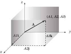
Any vector $\bold{A}$ in 3 dimensions can be represented with initial point at the origin O of a rectangular coordinate system. Let $(A_1, A_2, A_3)$ be the rectangular coordinates of the terminal point of vector $\bold{A}$ with initial point at O. The vectors $A_1\bold{i}$ , $A_2\bold{j}$ and $A_3\bold{k}$ are called the rectangular component vectors, or simply component vectors, of $\bold{A}$ in the x, y and z directions respectively. $A_1$ , $A_2$ and $A_3$ are called the rectangular components, or simply components, of $\bold{A}$ in the x, y and z directions respectively.

The sum or resultant of $A_1\bold{i}$ , $A_2\bold{j}$ and $A_3\bold{k}$ is the vector $\bold{A}$ , so that we can write
$\bold{A} = A_1\bold{i} + A_2\bold{j} + A_3\bold{k}\cdots(1)$
The magnitude of $\bold{A}$ is
$A = |\bold{A}| = \sqrt{A_1^2 + A_2^2 + A_3^2}\cdots(2)$
In particular, the position vector or radius vector $\bold{r}$ from O to the point (x, y, z) is written
$\bold{r} = x\bold{i} + y\bold{j} + z\bold{k}\cdots(3)$
and has magnitude $r = |\bold{r}| = \sqrt{x^2 + y^2 + z^2}$ .

ベクトルの成分

　3次元におけるいかなるベクトル $\bold{A}$ も直交座標系の原点 O における始点により表現可能です．ここでベクトル $\bold{A}$ を直交座標系における原点 O を始点とし $(A_1, A_2, A_3)$ を終点としましょう．そのベクトル $A_1\bold{i}$ , $A_2\bold{j}$ および $A_3\bold{k}$ はそれぞれ $\bold{A}$ における x, y および z 軸方向の 直交成分ベクトル, あるいは単に 成分ベクトル といいます． $A_1$ , $A_2$ および $A_3$ はそれぞれ x, y および z 軸方向における $\bold{A}$ の 直交成分, または単に成分と呼ばれます．

　 $A_1\bold{i}$ , $A_2\bold{j}$ および $A_3\bold{k}$ の和や結果が $\bold{A}$ であり，ゆえに

$\bold{A} = A_1\bold{i} + A_2\bold{j} + A_3\bold{k}\cdots(1)$

　 $\bold{A}$ の大きさは

$A = |\bold{A}| = \sqrt{A_1^2 + A_2^2 + A_3^2}\cdots(2)$

　特に，原点 O から点 (x, y, z) への 位置ベクトル または 動径ベクトル $\bold{r}$ は以下のように記述できます．

$\bold{r} = x\bold{i} + y\bold{j} + z\bold{k}\cdots(3)$

またその大きさは $r = |\bold{r}| = \sqrt{x^2 + y^2 + z^2}$ となります．

Rectangular unit vectors

The rectangular unit vectors $\bold{i}$ , $\bold{j}$ and $\bold{k}$ are unit vectors having the direction of the positive x, y, and z axes of a rectangular coordinate system. We use right-handed rectangular coordinate system unless otherwise specified. Such systems derive their name from the fact that a right threaded screw rotated through 90° from Ox to Oy will advance in the positive z direction. In general, three vectors $\bold{A}$ , $\bold{B}$ and $\bold{C}$ which have coincident initial points and are not coplanar are said to form a right-handed system if a right threaded screw rotated through an angle less than 180° from $\bold{A}$ to $\bold{B}$ will advance in the direction $\bold{C}$ .

直交単位ベクトル

　直交単位ベクトルは直交座標系におけるx軸y軸z軸の正の方向を有する単位ベクトルです．今後特に断らない限り，右手の直交座標系を用いることにします．そのような系の名は右巻きのねじが Ox から Oy に90°回転すると z 軸の正方向に進むことに由来します．一般的に3つのベクトル $\bold{A}$ , $\bold{B}$ , $\bold{C}$ が一致した始点を有し，かつ同一平面上にないものは，もし $\bold{A}$ から $\bold{B}$ まで 180° 以内に回転する右巻きねじが $\bold{C}$ 方向に進行するなら，右手系 または 右巻き系 を形成すると言います．

月	火	水	木	金	土	日
		1	2	3	4	5
6	7	8	9	10	11	12
13	14	15	16	17	18	19
20	21	22	23	24	25	26
27	28	29	30	31