EXCEL のワークシートに挿入されたテーブルにはデフォルトでオートフィルターが設定されています.このテーブルに対してオートフィルターをかけた結果を VBA で取得する方法は難解で,従来の考え方とは少し異なります.
より抽象度の高い考え方をする必要があります.リレーショナルデータベースの概念である集合論を理解する必要があります.
with Database, Statistics and Nutrition

EXCEL のワークシートに挿入されたテーブルにはデフォルトでオートフィルターが設定されています.このテーブルに対してオートフィルターをかけた結果を VBA で取得する方法は難解で,従来の考え方とは少し異なります.
より抽象度の高い考え方をする必要があります.リレーショナルデータベースの概念である集合論を理解する必要があります.
EXCEL は散布図を描く際によく用いています.散布図のデータ系列の指定は奥深く,非常に難しいものがあり,少し凝ったことをしようとすると大変な目に遭います.
手動では設定不可能なほどの数のデータ系列の設定を VBA から行えないか,試行錯誤しました.今回はマクロの記録にとどめます.
総務省の都道府県・市区町村別統計表は 5 年毎に施行される国勢調査を元に作成されており,日本の人口統計の基本となる資料です.
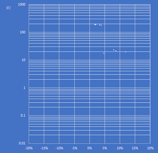
今回はこの資料を元に人口と人口増減率を散布図にするため第一正規形にします.
森林を構成する樹木の分布と積算温度には対応が見られます.暖かい地方では冬の寒さが,寒い地方では夏の暑さが植物の分布を制約するためです.吉良竜夫はこの点に注目し,暖かさの指数warmth indexおよび寒さの指数coldness indexという温量指数を考案しました.
暖かさの指数とは『月平均気温が5℃を越す月の平均気温から5℃を引いた値の合計』です.寒さの指数とは『月平均気温が5℃未満の月について,月の平均気温と5℃との差の合計』でマイナスをつけて表現します.温量指数と言う場合,普通は暖かさの指数を指します.
日本の植生帯を特徴づける樹木の分布帯と暖かさの指数との関係をみると,180, 85, 45, 15のところにそれぞれの植生帯の上端(すなわち低温側の分布限界)が集中していると言われます.それに基づいて日本の気候は次のように分類されます.
気象庁のサイトでは日本全国の過去の気象データを蓄積しており,それらをダウンロードすることができます.今回は EXCEL VBA を用いて Web Query によりデータをダウンロードし,温量指数を計算する方法を述べます.
方法はこちらのページ(EXCEL VBAで気象庁ホームページから風向風速,降水量,気温,日照時間のデータをダウンロードする)に詳しいですが,同ページのコードが動かなかったため,再度マクロの記録から接続文字列などを検証しました.
まずは手動でダウンロードする場合です.気象庁の過去の気象データ検索ページを開きます.地点,年月日,データの種類で絞り込みます.任意の地点を選択します.ここで必要なのは月平均気温ですので,年月日は年を指定し,月と日は指定せずにおきます.データの種類は『****年の月ごとの値を表示』です.
ここでブラウザのURLを取得します.
https://www.data.jma.go.jp/obd/stats/etrn/view/monthly_a1.php?prec_no=55&block_no=0552&year=1977&month=&day=&view=p1
year= で年を指定しており,ここを変数化してループすればEXCELでデータを自動抽出できます.以下コードです.
Option Explicit

Sub WarmthIndex()

Dim mySht               As Worksheet
Dim myWeather(1048574, 15)  As Variant
Dim myURL               As String
Dim myYear              As Integer
Dim myMonth             As Integer
Dim myDate              As Date
Dim myRng               As Range
Dim myPlace             As String
Dim i                   As Integer
Dim j                   As Long
Dim myTime              As Single

    Application.ScreenUpdating = False
    j = 0
    myDate = Date
    myPlace = "**"
    myTime = Timer

    For myYear = 1977 To Year(myDate) - 1

        myURL = "URL;https://www.data.jma.go.jp/obd/stats/etrn/view/monthly_a1.php?prec_no=55&block_no=0552&year=" & myYear & "&month=&day=&view=p1"
        Set mySht = Worksheets.Add
        Set myRng = mySht.Range("$A$1")

        With mySht.QueryTables.Add(Connection:=myURL, Destination:=myRng)
            .WebSelectionType = xlSpecifiedTables
            .WebFormatting = xlWebFormattingNone
            .WebTables = """tablefix1"""
            .Refresh BackgroundQuery:=False
        End With

        Set myRng = myRng.CurrentRegion
        With myRng
            .Replace What:=" ", Replacement:=""
            .Replace What:="]", Replacement:=""
            .Replace What:=")", Replacement:=""
            .Replace What:="/", Replacement:=""
        End With

        For i = 0 To myRng.Rows.Count - 4
            myWeather(j, 0) = myPlace
            myWeather(j, 1) = myYear
            myWeather(j, 2) = myRng(i + 4, 1)
            myWeather(j, 3) = myRng(i + 4, 2)
            myWeather(j, 4) = myRng(i + 4, 3)
            myWeather(j, 5) = myRng(i + 4, 4)
            myWeather(j, 6) = myRng(i + 4, 6)
            myWeather(j, 7) = myRng(i + 4, 7)
            myWeather(j, 8) = myRng(i + 4, 8)
            myWeather(j, 9) = myRng(i + 4, 9)
            myWeather(j, 10) = myRng(i + 4, 10)
            myWeather(j, 11) = myRng(i + 4, 11)
            myWeather(j, 12) = myRng(i + 4, 12)
            myWeather(j, 13) = myRng(i + 4, 13)
            myWeather(j, 14) = myRng(i + 4, 16)
            Select Case True
            Case myRng(i + 4, 6) - 5 <= 0
                myWeather(j, 15) = 0
            Case Else
                myWeather(j, 15) = myRng(i + 4, 6) - 5
            End Select
            j = j + 1
        Next i

        Application.DisplayAlerts = False
        mySht.Delete
        Application.DisplayAlerts = True

    Next myYear

    Set mySht = Worksheets.Add
    With mySht
        .Name = myYear & myPlace & "温量指数"
        .Range("$A$1") = "地点"
        .Range("$B$1") = "年"
        .Range("$C$1") = "月"
        .Range("$D$1") = "降水量合計"
        .Range("$E$1") = "日最大降水量"
        .Range("$F$1") = "1時間最大降水量"
        .Range("$G$1") = "日平均気温"
        .Range("$H$1") = "日最高気温"
        .Range("$I$1") = "日最低気温"
        .Range("$J$1") = "最高気温"
        .Range("$K$1") = "最低気温"
        .Range("$L$1") = "平均風速"
        .Range("$M$1") = "最大風速"
        .Range("$N$1") = "最大風向"
        .Range("$O$1") = "日照時間"
        .Range("$P$1") = "温量指数"
        .Range("$A$2:$P$1048576") = myWeather
    End With

    Debug.Print Round(Timer - myTime, 2)
    Set myRng = Nothing
    Set mySht = Nothing
    Application.ScreenUpdating = True

End Sub
ピボットテーブルを挿入します.設定はデフォルトで結構です.『行』には年をドラッグします.『値』には温量指数をドラッグします.『集計方法』はデータの合計です.これで温量指数が算出されます.
グラフを追加するなら折れ線グラフが良いでしょう.下図は当地の温量指数の推移ですが,1987年までは95から105の範囲を推移していたのが,1988年から2004年までは95から115までの範囲を乱高下を繰り返し,2005年以降は110近辺の範囲に収まってきているように見えます.全体として温暖化傾向が見られます.

次に,夏枯れ指数を算出します.夏枯れ指数とは『日最高気温が25℃を超えた日について25℃との差を年間で合計した値』(武井和久)のことです.基準とした25℃は寒地型芝草が弱り始める温度です.コードのみ載せます.
Option Explicit

Sub SummerSlumpIndex()

Dim mySht               As Worksheet
Dim myWeather(1048574, 13)  As Variant
Dim myURL               As String
Dim myYear              As Integer
Dim myMonth             As Integer
Dim myDate              As Date
Dim myRng               As Range
Dim myPlace             As String
Dim i                   As Integer
Dim j                   As Long
Dim myTime              As Single

    Application.ScreenUpdating = False
    j = 0
    myDate = Date
    myPlace = "**"
    myTime = Timer

    For myYear = 1977 To Year(myDate) - 1

        On Error Resume Next
        If DateSerial(myYear, myMonth, 1) - DateSerial(Year(myDate), Month(myDate), 1) >= 0 Then
            Exit For
        End If
        On Error GoTo 0

        For myMonth = 1 To 12

            myURL = "URL;https://www.data.jma.go.jp/obd/stats/etrn/view/daily_a1.php?prec_no=55&block_no=0552&year=" & myYear & "&month=" & myMonth & "&day=&view=p1"
            Set mySht = Worksheets.Add
            Set myRng = mySht.Range("$A$1")

            With mySht.QueryTables.Add(Connection:=myURL, Destination:=myRng)
                .WebSelectionType = xlSpecifiedTables
                .WebFormatting = xlWebFormattingNone
                .WebTables = """tablefix1"""
                .Refresh BackgroundQuery:=False
            End With

            Set myRng = myRng.CurrentRegion
            With myRng
                .Replace What:=" ", Replacement:=""
                .Replace What:="]", Replacement:=""
                .Replace What:=")", Replacement:=""
                .Replace What:="/", Replacement:=""
            End With

            For i = 0 To myRng.Rows.Count - 4
                myWeather(j, 0) = myPlace
                myWeather(j, 1) = DateSerial(myYear, myMonth, myRng(i + 4, 1))
                myWeather(j, 2) = myRng(i + 4, 2)
                myWeather(j, 3) = myRng(i + 4, 3)
                myWeather(j, 4) = myRng(i + 4, 5)
                myWeather(j, 5) = myRng(i + 4, 6)
                myWeather(j, 6) = myRng(i + 4, 7)
                myWeather(j, 7) = myRng(i + 4, 8)
                myWeather(j, 8) = myRng(i + 4, 9)
                myWeather(j, 9) = myRng(i + 4, 10)
                myWeather(j, 10) = myRng(i + 4, 13)
                myWeather(j, 11) = myRng(i + 4, 14)
                Select Case True
                Case myRng(i + 4, 5) - 5 <= 0
                    myWeather(j, 12) = 0
                Case Else
                    myWeather(j, 12) = myRng(i + 4, 5) - 5
                End Select
                Select Case True
                Case myRng(i + 4, 6) - 25 <= 0
                    myWeather(j, 13) = 0
                Case Else
                    myWeather(j, 13) = myRng(i + 4, 6) - 25
                End Select
                j = j + 1
            Next i

            Application.DisplayAlerts = False
            mySht.Delete
            Application.DisplayAlerts = True

        Next myMonth
    Next myYear

    Set mySht = Worksheets.Add
    With mySht
        .Name = myYear & myPlace
        .Range("$A$1") = "地点"
        .Range("$B$1") = "年月日"
        .Range("$C$1") = "降水量合計"
        .Range("$D$1") = "1時間最大降水量"
        .Range("$E$1") = "平均気温"
        .Range("$F$1") = "最高気温"
        .Range("$G$1") = "最低気温"
        .Range("$H$1") = "平均風速"
        .Range("$I$1") = "最大風速"
        .Range("$J$1") = "最大風向"
        .Range("$K$1") = "最多風向"
        .Range("$L$1") = "日照時間"
        .Range("$M$1") = "温量指数"
        .Range("$N$1") = "夏枯れ指数"
        .Range("$A$2:$N$1048576") = myWeather
    End With

    Debug.Print Round(Timer - myTime, 2)
    Set myRng = Nothing
    Set mySht = Nothing
    Application.ScreenUpdating = True

End Sub
ピボットテーブルを挿入します.『行』には年月日をドラッグします.『値』には夏枯れ指数をドラッグします.『集計方法』はデータの合計です.更に『分析』タブの『グループの選択』コマンドをクリックし,『グループ化』ウィンドウで『年』のみを選択して年月日を集約します.これで夏枯れ指数が算出されます.同様に温暖化傾向が見られます.

In this article, I’d like to describe how to fix the text file of the food composition of the diet recipes, which a facility have provided for one year, to the first normal form in order to insert into database.
Option Explicit

Sub LoopProcedure()
    Dim Sh  As Worksheet
    For Each Sh In Worksheets
        If Sh.Name Like "Sheet" & "*" Then
            Call TransportFromTxtToCSV(Sh)
        End If
    Next Sh
End Sub

Sub TransportFromTxtToCSV()
    Dim mySht               As Worksheet
    Dim myRng               As Range
    Dim myAr                As Variant
    Dim RecAr()             As String
    Dim i                   As Long
    Dim j                   As Long
    Dim k                   As Long
    Dim Date_Serving_Meal   As Date
    Dim Menu_Name           As String
    Dim tmpStart            As Long
    Dim Meal_Time           As String
    Dim Dish                As String
    Dim RecordNumber        As Long

    set mysht = sh
    RecordNumber = Count_Record(mySht)
    ReDim RecAr(RecordNumber - 1, 51)
    Set myRng = mySht.UsedRange
    myAr = myRng
    k = 0
    Date_Serving_Meal = "2011/1/1"
    Menu_Name = myAr(1, 11) & myAr(1, 12) & myAr(1, 13)
    tmpStart = InStr(Menu_Name, ")")
    Menu_Name = Mid(Menu_Name, tmpStart + 1)
    Meal_Time = "朝食"
    For i = LBound(myAr) To UBound(myAr)

        Select Case True
            Case myAr(i, 2) = "合      計"
                Date_Serving_Meal = DateAdd("d", 1, Date_Serving_Meal)
            Case myAr(i, 2) = "《朝食》"
                Meal_Time = "朝食"
            Case myAr(i, 2) = "《昼食》"
                Meal_Time = "昼食"
            Case myAr(i, 2) = "《夕食》"
                Meal_Time = "夕食"
            Case myAr(i, 2) = "小      計"
            Case myAr(i, 2) = "^e12【献立"
            Case myAr(i, 2) Like "動蛋比" & "*"
            Case myAr(i, 2) = "・・・・・・・・・・"
            Case myAr(i, 2) = "料理名"
            Case myAr(i, 2) = ""
            Case Else
                Dish = myAr(i, 2)
        End Select

        Select Case True
            Case myAr(i, 3) = "・・・・・・・・・・・"
            Case myAr(i, 3) Like "EN比" & "*"
            Case myAr(i, 3) = "食品名"
            Case myAr(i, 3) Like "一覧表】 ^e11" & "*"
            Case myAr(i, 3) = ""
            Case Else
                RecAr(k, 0) = Date_Serving_Meal
                RecAr(k, 1) = Menu_Name
                RecAr(k, 2) = Meal_Time
                RecAr(k, 3) = Dish
                RecAr(k, 4) = myAr(i, 3)
                For j = 5 To 22
                    RecAr(k, j) = myAr(i, j - 1)
                Next j
                For j = 23 To 39
                    RecAr(k, j) = myAr(i + 1, j - 18)
                Next j
                For j = 40 To 51
                    RecAr(k, j) = myAr(i + 2, j - 35)
                Next j
                k = k + 1
        End Select
    Next i
    Set mySht = Worksheets.Add
    With mySht
        .Name = Menu_Name
        .Range(Cells(1, 1), Cells(RecordNumber, 52)) = RecAr
    End With

    Set mySht = Nothing
    Set myRng = Nothing
    Erase RecAr
End Sub

Function Count_Record(ByRef Sh As Worksheet) As Long
    Dim mySht       As Worksheet
    Dim myAr        As Variant
    Dim i           As Long
    Dim j           As Long
    Dim k           As Long
    Set mySht = Sh
    myAr = mySht.UsedRange
    j = 0
    k = 0
    For i = LBound(myAr) To UBound(myAr)
        Select Case True
            Case myAr(i, 2) = "合      計"
            Case myAr(i, 2) = "小      計"
            Case myAr(i, 2) = "《朝食》"
            Case myAr(i, 2) = "《昼食》"
            Case myAr(i, 2) = "《夕食》"
            Case myAr(i, 2) = "^e12【献立"
            Case myAr(i, 2) Like "動蛋比" & "*"
            Case myAr(i, 2) = "・・・・・・・・・・"
            Case myAr(i, 2) = "料理名"
            Case myAr(i, 2) = ""
            Case Else
                j = j + 1
        End Select
        Select Case True
            Case myAr(i, 3) = "・・・・・・・・・・・"
            Case myAr(i, 3) Like "EN比" & "*"
            Case myAr(i, 3) = "食品名"
            Case myAr(i, 3) Like "一覧表】 ^e11" & "*"
            Case myAr(i, 3) = ""
            Case Else
                k = k + 1
        End Select
    Next i
    Count_Record = k
End Function
ある施設の1年間で提供した食事のレシピの食品成分のテキストファイルから,データベースに取り込むための前処置としてデータを第1正規形に整形する EXCEL VBA コードです.個人的な備忘録です.
94行目以降の関数 Count_Record は,アクティブシートをループして必要なレコード数を計測する関数です.104行目以降で料理名の数(B列),119行目以降で食品名の数(C列)に注目しています.サブルーチン TransportFromTxtToCSV から呼び出して,動的配列の要素数を後で決定するのに用います.
Option Explicit

Sub LoopProcedure()
    Dim Sh  As Worksheet
    For Each Sh In Worksheets
        If Sh.Name Like "Sheet" & "*" Then
            Call TransportFromTxtToCSV(Sh)
        End If
    Next Sh
End Sub

Sub TransportFromTxtToCSV()
    Dim mySht               As Worksheet
    Dim myRng               As Range
    Dim myAr                As Variant
    Dim RecAr()             As String
    Dim i                   As Long
    Dim j                   As Long
    Dim k                   As Long
    Dim Date_Serving_Meal   As Date
    Dim Menu_Name           As String
    Dim tmpStart            As Long
    Dim Meal_Time           As String
    Dim Dish                As String
    Dim RecordNumber        As Long

    set mysht = sh
    RecordNumber = Count_Record(mySht)
    ReDim RecAr(RecordNumber - 1, 51)
    Set myRng = mySht.UsedRange
    myAr = myRng
    k = 0
    Date_Serving_Meal = "2011/1/1"
    Menu_Name = myAr(1, 11) & myAr(1, 12) & myAr(1, 13)
    tmpStart = InStr(Menu_Name, ")")
    Menu_Name = Mid(Menu_Name, tmpStart + 1)
    Meal_Time = "朝食"
    For i = LBound(myAr) To UBound(myAr)

        Select Case True
            Case myAr(i, 2) = "合      計"
                Date_Serving_Meal = DateAdd("d", 1, Date_Serving_Meal)
            Case myAr(i, 2) = "《朝食》"
                Meal_Time = "朝食"
            Case myAr(i, 2) = "《昼食》"
                Meal_Time = "昼食"
            Case myAr(i, 2) = "《夕食》"
                Meal_Time = "夕食"
            Case myAr(i, 2) = "小      計"
            Case myAr(i, 2) = "^e12【献立"
            Case myAr(i, 2) Like "動蛋比" & "*"
            Case myAr(i, 2) = "・・・・・・・・・・"
            Case myAr(i, 2) = "料理名"
            Case myAr(i, 2) = ""
            Case Else
                Dish = myAr(i, 2)
        End Select

        Select Case True
            Case myAr(i, 3) = "・・・・・・・・・・・"
            Case myAr(i, 3) Like "EN比" & "*"
            Case myAr(i, 3) = "食品名"
            Case myAr(i, 3) Like "一覧表】 ^e11" & "*"
            Case myAr(i, 3) = ""
            Case Else
                RecAr(k, 0) = Date_Serving_Meal
                RecAr(k, 1) = Menu_Name
                RecAr(k, 2) = Meal_Time
                RecAr(k, 3) = Dish
                RecAr(k, 4) = myAr(i, 3)
                For j = 5 To 22
                    RecAr(k, j) = myAr(i, j - 1)
                Next j
                For j = 23 To 39
                    RecAr(k, j) = myAr(i + 1, j - 18)
                Next j
                For j = 40 To 51
                    RecAr(k, j) = myAr(i + 2, j - 35)
                Next j
                k = k + 1
        End Select
    Next i
    Set mySht = Worksheets.Add
    With mySht
        .Name = Menu_Name
        .Range(Cells(1, 1), Cells(RecordNumber, 52)) = RecAr
    End With

    Set mySht = Nothing
    Set myRng = Nothing
    Erase RecAr
End Sub

Function Count_Record(ByRef Sh As Worksheet) As Long
    Dim mySht       As Worksheet
    Dim myAr        As Variant
    Dim i           As Long
    Dim j           As Long
    Dim k           As Long
    Set mySht = Sh
    myAr = mySht.UsedRange
    j = 0
    k = 0
    For i = LBound(myAr) To UBound(myAr)
        Select Case True
            Case myAr(i, 2) = "合      計"
            Case myAr(i, 2) = "小      計"
            Case myAr(i, 2) = "《朝食》"
            Case myAr(i, 2) = "《昼食》"
            Case myAr(i, 2) = "《夕食》"
            Case myAr(i, 2) = "^e12【献立"
            Case myAr(i, 2) Like "動蛋比" & "*"
            Case myAr(i, 2) = "・・・・・・・・・・"
            Case myAr(i, 2) = "料理名"
            Case myAr(i, 2) = ""
            Case Else
                j = j + 1
        End Select
        Select Case True
            Case myAr(i, 3) = "・・・・・・・・・・・"
            Case myAr(i, 3) Like "EN比" & "*"
            Case myAr(i, 3) = "食品名"
            Case myAr(i, 3) Like "一覧表】 ^e11" & "*"
            Case myAr(i, 3) = ""
            Case Else
                k = k + 1
        End Select
    Next i
    Count_Record = k
End Function
In order to validate multicollinearity in multivariate analysis, you could investigate signs of partial correlation matrix. You could calculate partial correlation coefficient, rij rest, when you would be given covariates without xi and xj and it’s assumed that R = (rij) as correlation matrix and R-1 = (rij) as inverse matrix, respectively.
Reverse the sign of the elements divided by square of products of the diagonal elements, they are partial correlation coefficients. The set of partial correlation coefficients is partial correlation matrix.
When the signs didn’t match between correlation matrix and partial correlation matrix, it suggests multicollinearity. When there was linear relationship between covariates, inverse matrix of correlation matrix could not be obtained.
You could get partial correlation matrix as below. It’s assumed that you have already get correlation matrix.
| A | B | C | |
| 1 | 1.000 | 0.800 | 0.300 |
| 2 | 0.800 | 1.000 | -0.700 |
| 3 | 0.300 | -0.700 | 1.000 |
Excel has worksheet function to get inverse matrix. You need to press the Control key, Shift key and Enter key at the same time when you confirm the argument as MINVERSE function.
{=MINVERS($A$1:$C$3)}
| A | B | C | |
| 5 | -0.197 | 1.817 | 1.547 |
| 6 | 1.817 | -1.637 | -1.691 |
| 7 | 1.547 | -1.691 | -0.647 |
You would have to use INDEX function, ROW function and COLUMN function. Paste following formula to the corresponding cells. The number subtracted from the return of ROW function (and COLUMN function) would change depending on the situation.
=-INDEX($A$5:$C$7, ROW()-8,COLUMN())/SQRT(INDEX($A$5:$C$7, ROW()-8, ROW()-8)*INDEX($A$5:$C$7, COLUMN(),COLUMN()))
| A | B | C | |
| 9 | 1.000 | -1.483 | -2.007 |
| 10 | -1.483 | 1.000 | 1.642 |
| 11 | -2.007 | 1.642 | 1.000 |
多変量解析において変数間の多重共線性を調べる方法の一つに偏相関行列があります.相関行列を R = (rij) とし,その逆行列を R-1 = (rij) とすると,xi と xj 以外のすべての変数を与えた時の xi と xj の偏相関係数 rij rest は下式で表現できます.
逆行列の対応する要素を2つの対角要素の積の平方根で割って基準化し,符号を反転します.この偏相関係数を全ての変数の対について行列の形にまとめたものを偏相関行列と言います.
相関行列と偏相関行列の符号が一致しない場合は多重共線性の可能性があります.また,変数間に線形の関係がある場合は相関行列の逆行列が求まらないこともあります.
Excelで偏相関行列を求める方法は下記の通りです.既に相関行列は求まっているものとします.
| A | B | C | |
| 1 | 1.000 | 0.800 | 0.300 |
| 2 | 0.800 | 1.000 | -0.700 |
| 3 | 0.300 | -0.700 | 1.000 |
逆行列を求めるワークシート関数は Excel に標準装備されています.MINVERS 関数を用いる時の注意点として,関数の引数として相関行列を指定し,確定する際に Control キーと Shift キーと Enter キーを同時に押下する必要があります.
{=MINVERS($A$1:$C$3)}
| A | B | C | |
| 5 | -0.197 | 1.817 | 1.547 |
| 6 | 1.817 | -1.637 | -1.691 |
| 7 | 1.547 | -1.691 | -0.647 |
求まった逆行列の各要素から2つの対角要素のアドレスを求めるには少々工夫が必要です.INDEX 関数と ROW 関数および COLUMN 関数を組み合わせます.下式を該当セルにペーストします.ROW 関数(および COLUMN 関数)から差し引いている数値は INDEX 関数の第 1 引数の 2 次元配列の行番号(と列番号)を指定するものですので,状況によって数値は変化します.各自で対応して下さい.
=-INDEX($A$5:$C$7, ROW()-8,COLUMN())/SQRT(INDEX($A$5:$C$7, ROW()-8, ROW()-8)*INDEX($A$5:$C$7, COLUMN(),COLUMN()))
| A | B | C | |
| 9 | 1.000 | -1.483 | -2.007 |
| 10 | -1.483 | 1.000 | 1.642 |
| 11 | -2.007 | 1.642 | 1.000 |
You may use Akaike information criterion (AIC) to evaluate fitting of multivariate model. You could use c-index that Harrell have proposed. Although it seems to evaluate fitting of present data set, it seems not to consider about future data set, it might result in overfitting to present data set.
It’s assumed that sample size is N, the number of pairs could be calculated following formula.
It’s assumed that worksheet’s structure follows the list below.
Option Explicit

Sub C_Statistics()
    Dim i   As Long
    Dim j   As Long
    Dim k   As Long
    Dim Rng As Range
    Dim Ar  As Variant
    k = 0
    Set Rng = ActiveSheet.UsedRange
    Set Rng = Rng.Resize(Rng.Rows.Count - 1).Offset(1)
    Ar = Rng
    For i = LBound(Ar) To UBound(Ar) - 1
        For j = i + 1 To UBound(Ar)
            k = k + 1
        Next j
    Next i
    Debug.Print "k= " & k
End Sub
Risk score (R) is calculated as following formula.
A point estimated of effect size in COX proportional hazard analysis is hazard ratio (Exp(Β)) and regression coefficient of covariate is logarithm of hazard ratio (Β). It’s assumed that risk score has been calculated.
It’s important that “If both of pair was censored or one of pair was censored and survival time of censored is short, they were classified as unknown”. In other words,
It’s as following VBA code. It’s assumed that it doesn’t includes equal sign if both survival time of pair were equal.
            Select Case Ar(i, 2) + Ar(j, 2)
            Case 0
                k = k + 1
            Case 1
                If (Ar(i, 1) - Ar(j, 1)) * (Ar(i, 2) - Ar(j, 2)) > 0 Then
                    k = k + 1
                End If
            End Select
Furthermore, you would compare risk score and survival time between both of pair and evaluate the sign of product of the differentiation of risk score and the differentiation of survival time, respectively. It means that whether the magnitude of risk score and the length of survival time are consistent or not. It’s assumed that lower risk score means longer survival time.
Option Explicit

Sub C_Statistics()
    Dim i   As Long
    Dim j   As Long
    Dim k   As Long
    Dim n1  As Long
    Dim n2  As Long
    Dim n3  As Long
    Dim Rng As Range
    Dim Ar  As Variant

    k = 0
    n1 = 0
    n2 = 0
    n3 = 0
    Set Rng = ActiveSheet.UsedRange
    Set Rng = Rng.Resize(Rng.Rows.Count - 1).Offset(1)
    Ar = Rng
    For i = LBound(Ar) To UBound(Ar) - 1
        For j = i + 1 To UBound(Ar)
            Select Case Ar(i, 2) + Ar(j, 2)
            Case 0
                If (Ar(i, 1) - Ar(j, 1)) * (Ar(i, 3) - Ar(j, 3)) < 0 Then
                    n1 = n1 + 1
                End If
                If (Ar(i, 1) - Ar(j, 1)) * (Ar(i, 4) - Ar(j, 4)) < 0 Then
                    n2 = n2 + 1
                End If
                If (Ar(i, 1) - Ar(j, 1)) * (Ar(i, 5) - Ar(j, 5)) < 0 Then
                    n3 = n3 + 1
                End If
                k = k + 1
            Case 1
                If (Ar(i, 1) - Ar(j, 1)) * (Ar(i, 2) - Ar(j, 2)) > 0 Then
                    If (Ar(i, 1) - Ar(j, 1)) * (Ar(i, 3) - Ar(j, 3)) < 0 Then
                        n1 = n1 + 1
                    End If
                    If (Ar(i, 1) - Ar(j, 1)) * (Ar(i, 4) - Ar(j, 4)) < 0 Then
                        n2 = n2 + 1
                    End If
                    If (Ar(i, 1) - Ar(j, 1)) * (Ar(i, 5) - Ar(j, 5)) < 0 Then
                        n3 = n3 + 1
                    End If
                    k = k + 1
                End If
            End Select
        Next j
    Next i
    Debug.Print "n1= " & n1, "n2= " & n2, "n3= " & n3, "k= " & k
    Debug.Print "C1= " & n1 / k, "C2= " & n2 / k, "C3= " & n3 / k
End Sub
The sign of 35th line is larger than 0, it's assumed that censor is 1 and death is 0, would be reversed if censor was 0 and death was 1. The signs of 24th, 27th, 30th, 36th, 39th and 42nd would be reversed if it was assumed that higher risk score means longer survival time.
n1/k, n2/k and n3/k are c-index of model 1, model 2 and model 3, respectively. c-index ranges between 0 and 1. If c-index is 0.5, it means that the model doesn't fit at all. If it's closer to 0 or 1, it means that the model fits better.
Draw a pair of patients and determine which patient lived longer from his baseline evaluation. Survival times can be validly compared either when both patients have died, or when one has died and the other's followup time has exceeded the survival time of the first. If both patients are still alive, which will live longer is not known, and that pair of patients is not used in the analysis. Otherwise, it can be determined whether the patient with the higher prognostic score (ie, the weighted combination of baseline and test variables used to predict survival) also had the longer survival time. The process is repeated until all possible pairs of patients have been examined. Of the pairs of patients for which the ordering of survival time s could be inferred, the fraction of pairs such that the patient with the higher score had the longer survival time will be denoted by c.
The index c estimates the probability that, of two randomly chosen patients, the patient with the higher prognostic score will outlive the patient with the lower prognostic score. Values of c near .5 indicate that the prognostic score is no better than a coin-flip in determining which patient will live longer. Values of c near 0 or 1 indicate the baseline data virtually always determine which patient has a better prognosis. The c index measures a probability; many clinicians are more used to dealing with a correlation index that ranges from -1 to +1. A Kendall or Goodman-Kruskal type of correlation index can easily be constructed by calculating γ = 2(c - .5), where γ is the estimated probability that the prognostic score correctly orders prognosis for a pair of patients minus the probability that it incorrectly orders prognosis. When the prognostic score is unrelated to survival time, gamma is zero. When gamma = .5, the relationship between the prognostic score and survival time is halfway between a random relationship and a perfect relationship, and the corresponding c value is .75.
References:
Frank E. Harrell Jr, et al: Evaluating the Yield of Medical Tests. JAMA. 1982; 247 (18): 2543 - 2546
Morizane Toshio: Multivariate model, International Medical Information Center 2008; 29 (3): 8 - 12
多変量モデルの適合度の評価方法には通常赤池情報量基準 (AIC) を用いますが,Harrell らの提唱する c-index という指標もあります.c 統計値とも言い,リスクスコアの小さい(又は大きい)症例の方が生存期間が長いことが実際のデータでどれくらいの確率で正しいかを示す値です.方法は後述しますが,AIC と比較すると現在のデータに対する適合度のみを評価しており,未来のデータの予測精度への考慮がないように思えます.その意味で overfitting の可能性がある評価法と言えなくもありません.
サンプルサイズを N とすると,全てのペア数は下式で表現されます.
ワークシート上にデータがあるとして,1行が1症例とすると,全ての行から任意の2行を取り出すコードは下記のようになります.ワークシートの構造が以下のようであると仮定します.
Option Explicit

Sub C_Statistics()
    Dim i   As Long
    Dim j   As Long
    Dim k   As Long
    Dim Rng As Range
    Dim Ar  As Variant
    k = 0
    Set Rng = ActiveSheet.UsedRange
    Set Rng = Rng.Resize(Rng.Rows.Count - 1).Offset(1)
    Ar = Rng
    For i = LBound(Ar) To UBound(Ar) - 1
        For j = i + 1 To UBound(Ar)
            k = k + 1
        Next j
    Next i
    Debug.Print "k= " & k
End Sub
リスクスコア (R) は下式で表現されます.予後を規定するという意味で予後スコア prognostic score とも言います.β は回帰係数,X は共変量です.R0 は全症例のリスクスコアの平均値です.S0(t) はベースラインの生存率であり,全ての説明変数が基準値である場合の各時点 t での生存率です.
COX 比例ハザード分析では効果量の点推定値はハザード比 (Exp(Β)) として表現され,共変量の回帰係数はハザード比の対数 (LN(Exp(Β)) = Β) として表現します.それぞれの共変量にそれぞれの回帰係数をかけた積の和がリスクスコアです.ここでは既にリスクスコアの計算は終わっているものとします.
ここで重要な点は「2 症例とも打切例,あるいは片方が打切で打切までの期間がより短い場合は不明に分類される」との記述を条件式に表現する方法です.この条件は次のように言い換えることができます.
これを VBA で表現すると以下のようになります.2 行目と 4 行目の Case 式はそれぞれ上述した条件式に該当します.5 行目は上述の条件の後者を表現したものであり,生存期間の差と転帰の差との積を取り,符号が負の場合は拒否します.参照書籍の記述によると『打切例の打切までの生存期間が同じ値かあるいは短い場合にはどちらの生存が長いかは判断することができない』とのことですので,等号は外すこととします.
            Select Case Ar(i, 2) + Ar(j, 2)
            Case 0
                k = k + 1
            Case 1
                If (Ar(i, 1) - Ar(j, 1)) * (Ar(i, 2) - Ar(j, 2)) > 0 Then
                    k = k + 1
                End If
            End Select
さらにリスクスコアと生存期間とを比較します.同様にリスクスコアの差と生存期間の差との積の符号を評価します.リスクスコアの大小と生存期間の長短とが一致しているか否かを,差の積の符号に置き換えている訳です.最初に『リスクスコアの小さい(又は大きい)症例の方が生存期間が長いこと』と述べましたが,説明変数の設定によって各変数の係数の正負を逆転させ,リスクスコアの大小を逆転させることも可能です.ここではリスクスコアが小さいほど生存期間が長いという前提で話を進めます.
Option Explicit

Sub C_Statistics()
    Dim i   As Long
    Dim j   As Long
    Dim k   As Long
    Dim n1  As Long
    Dim n2  As Long
    Dim n3  As Long
    Dim Rng As Range
    Dim Ar  As Variant

    k = 0
    n1 = 0
    n2 = 0
    n3 = 0
    Set Rng = ActiveSheet.UsedRange
    Set Rng = Rng.Resize(Rng.Rows.Count - 1).Offset(1)
    Ar = Rng
    For i = LBound(Ar) To UBound(Ar) - 1
        For j = i + 1 To UBound(Ar)
            Select Case Ar(i, 2) + Ar(j, 2)
            Case 0
                If (Ar(i, 1) - Ar(j, 1)) * (Ar(i, 3) - Ar(j, 3)) < 0 Then
                    n1 = n1 + 1
                End If
                If (Ar(i, 1) - Ar(j, 1)) * (Ar(i, 4) - Ar(j, 4)) < 0 Then
                    n2 = n2 + 1
                End If
                If (Ar(i, 1) - Ar(j, 1)) * (Ar(i, 5) - Ar(j, 5)) < 0 Then
                    n3 = n3 + 1
                End If
                k = k + 1
            Case 1
                If (Ar(i, 1) - Ar(j, 1)) * (Ar(i, 2) - Ar(j, 2)) > 0 Then
                    If (Ar(i, 1) - Ar(j, 1)) * (Ar(i, 3) - Ar(j, 3)) < 0 Then
                        n1 = n1 + 1
                    End If
                    If (Ar(i, 1) - Ar(j, 1)) * (Ar(i, 4) - Ar(j, 4)) < 0 Then
                        n2 = n2 + 1
                    End If
                    If (Ar(i, 1) - Ar(j, 1)) * (Ar(i, 5) - Ar(j, 5)) < 0 Then
                        n3 = n3 + 1
                    End If
                    k = k + 1
                End If
            End Select
        Next j
    Next i
    Debug.Print "n1= " & n1, "n2= " & n2, "n3= " & n3, "k= " & k
    Debug.Print "C1= " & n1 / k, "C2= " & n2 / k, "C3= " & n3 / k
End Sub
35 行目の条件式の符号は打切が 1, 死亡が 0 の際のものです.打切が 0, 死亡が 1 なら符号は逆転します.同様にリスクスコアが大きいほど生存期間が長いなら 24, 27, 30, 36, 39, 42 行目の符号は逆転します.
リスクスコアと生存の関係が (1) 一致しているか,(2) 一致していないか,(3) 不明かで結果を場合分けしそれぞれの個数をカウントします.(1)/((1)+(2)) の比率が c-index です.上記では n1/k, n2/k, n3/k がそれぞれのモデルの c-index となります.c-index は 0 から 1 までの値を取りますが,0.5 の場合は全く適合していないと評価します.0 または 1 に近いほど適合が良いと評価します.
Draw a pair of patients and determine which patient lived longer from his baseline evaluation. Survival times can be validly compared either when both patients have died, or when one has died and the other's followup time has exceeded the survival time of the first. If both patients are still alive, which will live longer is not known, and that pair of patients is not used in the analysis. Otherwise, it can be determined whether the patient with the higher prognostic score (ie, the weighted combination of baseline and test variables used to predict survival) also had the longer survival time. The process is repeated until all possible pairs of patients have been examined. Of the pairs of patients for which the ordering of survival time s could be inferred, the fraction of pairs such that the patient with the higher score had the longer survival time will be denoted by c.
The index c estimates the probability that, of two randomly chosen patients, the patient with the higher prognostic score will outlive the patient with the lower prognostic score. Values of c near .5 indicate that the prognostic score is no better than a coin-flip in determining which patient will live longer. Values of c near 0 or 1 indicate the baseline data virtually always determine which patient has a better prognosis. The c index measures a probability; many clinicians are more used to dealing with a correlation index that ranges from -1 to +1. A Kendall or Goodman-Kruskal type of correlation index can easily be constructed by calculating γ = 2(c - .5), where γ is the estimated probability that the prognostic score correctly orders prognosis for a pair of patients minus the probability that it incorrectly orders prognosis. When the prognostic score is unrelated to survival time, gamma is zero. When gamma = .5, the relationship between the prognostic score and survival time is halfway between a random relationship and a perfect relationship, and the corresponding c value is .75.
参照:
Frank E. Harrell Jr, et al: Evaluating the Yield of Medical Tests. JAMA. 1982; 247 (18): 2543 - 2546
森實敏夫:多変量モデル,あいみっく,2008; 29 (3): 8 - 12(国際医学情報センター)
EXCEL VBA において,2 つの配列が等しいか否か調べたいことはよくあります.更に2つの配列の差分,つまり互いに重複しない要素を取り出したいという需要もあります.今回は配列の差分を求めるコードを紹介します.
2つの配列が等しいかをまず調べ,等しくない場合に次に一方が他方の真部分集合であるか否かを調べます.最後に配列の差分を求めます.この順になっているのは全く同じ2つの配列の差分は空集合となって解が求まらないためであり,引き算される配列が引き算する配列の真部分集合の場合にも結果が空集合となり解が求まらないためです.

Array1 の配列要素全体を A, Array2 の配列要素全体を B とすると Array1 から Array2 を差し引いた差分は下式で表現されます.
二重ループによりそれぞれの要素を比較して一致した数を求めていますが,これは積集合を取っていることに他なりません.EXCELワークシートにおいて数式の参照元の最初のセルおよび参照先の最後のセルを取得するでも述べましたが,2つの集合の和集合と積集合の要素数が等しければ元の2つの集合は全く同じです.ここでのロジックは積集合の要素数と元の集合の要素数が等しければ元の2つの集合は等しい筈であるとの前提に立っています.
Option Explicit

Function COMPARE_ARRAY(ByRef Array1() As String, ByRef Array2() As String) As Boolean
    Dim i   As Long
    Dim j   As Long
    Dim k   As Long
    k = 0
    For i = LBound(Array1) To UBound(Array1)
        For j = LBound(Array2) To UBound(Array2)
            If Array1(i) = Array2(j) Then
                k = k + 1
            End If
        Next j
    Next i
    If i = j And i = k Then
        COMPARE_ARRAY = True
    Else
        COMPARE_ARRAY = False
    End If
End Function

Function PROPERSUBSET_ARRAY(ByRef Array1() As String, ByRef Array2() As String) As Boolean
    Dim i   As Long
    Dim j   As Long
    Dim k   As Long
    k = 0
    For i = LBound(Array1) To UBound(Array1)
        For j = LBound(Array2) To UBound(Array2)
            If Array1(i) = Array2(j) Then
                k = k + 1
            End If
        Next j
    Next i
    If k = i Then
        PROPERSUBSET_ARRAY = True
    Else
        PROPERSUBSET_ARRAY = False
    End If
End Function
下記関数では第 3 引数の Compare の指定により Array1 から Array2 の差分を求めるか,Array2 から Array1 の差分を求めるかを指定しています.但し,配列内の要素にもともと空白文字列があった場合にはうまく動作しません.
Function EXCEPT_ARRAY(ByRef Array1() As String, ByRef Array2() As String, ByVal Compare As Boolean) As String()
    Dim i               As Long
    Dim j               As Long
    Dim k               As Long
    Dim InternalAr1()   As String
    Dim InternalAr2()   As String
    Dim Ar1Ar()         As String
    Dim Ar2Ar()         As String
    InternalAr1 = Array1
    InternalAr2 = Array2
    For i = LBound(InternalAr1) To UBound(InternalAr1)
        For j = LBound(InternalAr2) To UBound(InternalAr2)
            If InternalAr1(i) = InternalAr2(j) Then
                InternalAr1(i) = ""
                InternalAr2(j) = ""
                k = k + 1
            End If
        Next j
    Next i
    k = 0
    For i = LBound(InternalAr1) To UBound(InternalAr1)
        If InternalAr1(i) = "" Then
        Else
            ReDim Preserve Ar1Ar(k)
            Ar1Ar(k) = InternalAr1(i)
            k = k + 1
        End If
    Next i
    k = 0
    For j = LBound(InternalAr2) To UBound(InternalAr2)
        If InternalAr2(j) = "" Then
        Else
            ReDim Preserve Ar2Ar(k)
            Ar2Ar(k) = InternalAr2(j)
            k = k + 1
        End If
    Next j
    If Compare Then
        EXCEPT_ARRAY = Ar1Ar
    Else
        EXCEPT_ARRAY = Ar2Ar
    End If
End Function
参照:
EXCELワークシートにおいて数式の参照元の最初のセルおよび参照先の最後のセルを取得する
When you’d like to compare 2 arrays in EXCEL VBA whether they are equal or not, what would you do? Furthermore, you might get different elements that don’t overlap each other. I’d like to describe the code that how to get differences of 2 arrays.
At first, you would have to check whether they are equal each other or not because the difference of equal arrays is empty set. Next, you would have to check whether an array is proper subset of another array or not. At last, you could get difference between 2 arrays.
See formula as below, it is shown all elements of Array1 as “A”, all elements of Array2 as “B” and differences elements from Array1 and Array2 as “A And (not B)”.
The following code compares elements between two set and get number of equal elements with double loop, that means to get intersection of 2 sets.
Option Explicit

Function COMPARE_ARRAY(ByRef Array1() As String, ByRef Array2() As String) As Boolean
    Dim i   As Long
    Dim j   As Long
    Dim k   As Long
    k = 0
    For i = LBound(Array1) To UBound(Array1)
        For j = LBound(Array2) To UBound(Array2)
            If Array1(i) = Array2(j) Then
                k = k + 1
            End If
        Next j
    Next i
    If i = j And i = k Then
        COMPARE_ARRAY = True
    Else
        COMPARE_ARRAY = False
    End If
End Function

Function PROPERSUBSET_ARRAY(ByRef Array1() As String, ByRef Array2() As String) As Boolean
    Dim i   As Long
    Dim j   As Long
    Dim k   As Long
    k = 0
    For i = LBound(Array1) To UBound(Array1)
        For j = LBound(Array2) To UBound(Array2)
            If Array1(i) = Array2(j) Then
                k = k + 1
            End If
        Next j
    Next i
    If k = i Then
        PROPERSUBSET_ARRAY = True
    Else
        PROPERSUBSET_ARRAY = False
    End If
End Function
Configuration of the 3rd argument “Compare” specifies which array should be excepted, when it was TRUE the function would except the latter from the former, when it was FALSE then it would except the former from the latter, respectively. It’s assumed that the elements of arrays has no empty string.
Function EXCEPT_ARRAY(ByRef Array1() As String, ByRef Array2() As String, ByVal Compare As Boolean) As String()
    Dim i               As Long
    Dim j               As Long
    Dim k               As Long
    Dim InternalAr1()   As String
    Dim InternalAr2()   As String
    Dim Ar1Ar()         As String
    Dim Ar2Ar()         As String
    InternalAr1 = Array1
    InternalAr2 = Array2
    For i = LBound(InternalAr1) To UBound(InternalAr1)
        For j = LBound(InternalAr2) To UBound(InternalAr2)
            If InternalAr1(i) = InternalAr2(j) Then
                InternalAr1(i) = ""
                InternalAr2(j) = ""
                k = k + 1
            End If
        Next j
    Next i
    k = 0
    For i = LBound(InternalAr1) To UBound(InternalAr1)
        If InternalAr1(i) = "" Then
        Else
            ReDim Preserve Ar1Ar(k)
            Ar1Ar(k) = InternalAr1(i)
            k = k + 1
        End If
    Next i
    k = 0
    For j = LBound(InternalAr2) To UBound(InternalAr2)
        If InternalAr2(j) = "" Then
        Else
            ReDim Preserve Ar2Ar(k)
            Ar2Ar(k) = InternalAr2(j)
            k = k + 1
        End If
    Next j
    If Compare Then
        EXCEPT_ARRAY = Ar1Ar
    Else
        EXCEPT_ARRAY = Ar2Ar
    End If
End Function
オートフィルターの設定されているシートを手作業でフィルター解除するのは手間がかかります.VBA から GetOpenFilename メソッドで複数のブックを指定し,すべてのシートからオートフィルターを解除する方法です.
Option Explicit

Sub RemoveAutoFilter()
    Dim Wb      As Workbook
    Dim Sh      As Worksheet
    Dim myPath  As Variant
    Dim i       As Long
    Application.ScreenUpdating = False
    myPath = Application.GetOpenFilename(FileFilter:="Microsoft Excelブック,*.xls?", MultiSelect:=True)
    If TypeName(myPath) = "Boolean" Then Exit Sub
    For i = LBound(myPath) To UBound(myPath)
        Set Wb = Workbooks.Open(myPath(i))
        For Each Sh In Wb.Worksheets
            If Sh.AutoFilterMode Then
                Sh.AutoFilterMode = False
            End If
        Next Sh
        Wb.Save
        Wb.Close
    Next i
    Application.ScreenUpdating = True
End Sub
参照:
Application.GetOpenFilename メソッド (Excel)
It’s hard to remove manually AutoFilter of worksheets in multiple workbooks. I’d like to describe how to remove it with VBA.
Option Explicit

Sub RemoveAutoFilter()
    Dim Wb      As Workbook
    Dim Sh      As Worksheet
    Dim myPath  As Variant
    Dim i       As Long
    Application.ScreenUpdating = False
    myPath = Application.GetOpenFilename(FileFilter:="Microsoft Excel Book,*.xls?", MultiSelect:=True)
    If TypeName(myPath) = "Boolean" Then Exit Sub
    For i = LBound(myPath) To UBound(myPath)
        Set Wb = Workbooks.Open(myPath(i))
        For Each Sh In Wb.Worksheets
            If Sh.AutoFilterMode Then
                Sh.AutoFilterMode = False
            End If
        Next Sh
        Wb.Save
        Wb.Close
    Next i
    Application.ScreenUpdating = True
End Sub
Reference:
Application.GetOpenFilename Method (Excel)
It’s needed to enter password which requires a character, a number and a symbol at least, respectively. I’d like to describe how to validate password with VBScript®. It’s assumed that the length of password is 8 or greater.

In 23 line, the constraint is shown. In 22 line with comment, it’s shown that constrains password to require both a single-byte character and number at least and 8 or greater character length.
Option Explicit

Private Sub CommandButton1_Click()
    With TextBox1
        If Not CheckPassword(.Text) Then
            .SetFocus
            .SelStart = 0
            .SelLength = Len(.Text)
            Exit Sub
        Else

        End If
    End With
    Unload Me
End Sub

Function CheckPassword(InputString As String) As Boolean
    Dim myReg   As Object
    CheckPassword = False
    Set myReg = CreateObject("VBScript.RegExp")
    With myReg
       '.Pattern = "(?!^[0-9]*$)(?!^[a-zA-Z]*$)^([a-zA-Z0-9]{8,})$"
        .Pattern = "(?!^[0-9]*$)(?!^[a-zA-Z]*$)(?!^[!-/:-@[-`{-~]*$)(?!^[a-zA-Z0-9]*$)(?!^[!-@[-`{-~]*$)(?!^[!-/:-~]*$)^([!-~]{8,})$"
        .IgnoreCase = False
        .Global = True
    End With
    If myReg.Test(InputString) Then
        CheckPassword = True
    End If
    Set myReg = Nothing
End Function

Private Sub UserForm_Initialize()
    With TextBox1
        .IMEMode = fmIMEModeDisable
        .PasswordChar = "*"
    End With
End Sub
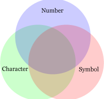
You might need description here. The pattern (?!pattern) means such negative lookahead as EXCEPT operator effects in SQL. To seek area three circles overlap, it’s needed to remove areas around. After filtering out not required patterns with negative lookahead, it validates length of the password. The number of required pattern, which verifies n types of letter, is 2n – 2.
| Not Needed | Negative Lookahead Pattern |
| Number | (?!^[0-9]*$) |
| Character | (?!^[a-zA-Z]*$) |
| Symbol | (?!^[!-/:-@[-`{-~]*$) |
| Character and number | (?!^[a-zA-Z0-9]*$) |
| Number and symbol | (?!^[!-@[-`{-~]*$) |
| Character and symbol | (?!^[!-/:-~]*$) |

References:
Regular Expression Language – Quick Reference
How To: Use Regular Expressions to Constrain Input in ASP.NET
ASCII character code list (0-127)
Userform of Excel VBA as user interface
パスワード設定の際に半角数字,半角英字,半角記号をそれぞれ最低でも 1 文字使用するよう求められるケースは多いと思います.今回は VBScript の正規表現を用いてパスワードをチェックする方法を紹介します.
制約条件を半角英数字,半角記号を最低でも 1 文字用いることとし,文字列長を 8 文字以上とします.下図のようにユーザーフォーム上にラベルとテキストボックスとコマンドボタンを配置します.それぞれ Label1, TextBox1, CommandButton1 とします.
下記コードの 23 行目で制約条件を表現します.コメントアウトした 22 行目は半角英数字のみを 8 文字以上用いる場合の正規表現です.文字クラス内でエスケープが必要なメタ文字は \ と ] の 2 種類です.
Option Explicit

Private Sub CommandButton1_Click()
    With TextBox1
        If Not CheckPassword(.Text) Then
            .SetFocus
            .SelStart = 0
            .SelLength = Len(.Text)
            Exit Sub
        Else

        End If
    End With
    Unload Me
End Sub

Function CheckPassword(InputString As String) As Boolean
    Dim myReg   As Object
    CheckPassword = False
    Set myReg = CreateObject("VBScript.RegExp")
    With myReg
       '.Pattern = "(?!^[0-9]*$)(?!^[a-zA-Z]*$)^([a-zA-Z0-9]{8,})$"
        .Pattern = "(?!^[0-9]*$)(?!^[a-zA-Z]*$)(?!^[!-/:-@[-`{-~]*$)(?!^[a-zA-Z0-9]*$)(?!^[!-@[-`{-~]*$)(?!^[!-/:-~]*$)^([!-~]{8,})$"
        .IgnoreCase = False
        .Global = True
    End With
    If myReg.Test(InputString) Then
        CheckPassword = True
    End If
    Set myReg = Nothing
End Function

Private Sub UserForm_Initialize()
    With TextBox1
        .IMEMode = fmIMEModeDisable
        .PasswordChar = "*"
    End With
End Sub
ここで解説が必要かと思います.(?!pattern) は否定先読みを示し,SQL で言うところの EXCEPT 演算子と同じ働きをします.半角英数字と半角記号を最低でも 1 文字以上使用するとは,下表の文字の組み合わせを許可しないということです.下図の 3 つの円の重なる領域を求めるには,その周辺の領域を引き算して求めます.許可しないパターンを否定先読みで予めフィルタリングしておき,最後に全種類の文字クラスの文字列長をチェックしています.集合論とも考え方の重なる領域です.ちなみに,n 種類の文字種を検証するのに必要な否定先読みのパターン数は 2n – 2 です.
| Not Needed | Negative Lookahead Pattern |
| Number | (?!^[0-9]*$) |
| Character | (?!^[a-zA-Z]*$) |
| Symbol | (?!^[!-/:-@[-`{-~]*$) |
| Character and number | (?!^[a-zA-Z0-9]*$) |
| Number and symbol | (?!^[!-@[-`{-~]*$) |
| Character and symbol | (?!^[!-/:-~]*$) |
参照:
ASP.NET への入力を制約するために正規表現を使用する方法
正規表現の構文
ASCII文字コード(0-127)一覧表
インターフェースとしてのEXCEL VBAによるユーザーフォーム
In the situation that you had to parse worksheet with much formula, what would you do? You would trace formula to first cell which has no reference. In this article, I’d like to describe to find the first cells with wading through spaghetti formula.
In order to demonstrate that set A is equal to set B, you should demonstrate that the union is equal to the intersection.
When you compare DirectPrecendents property and Precendents property, which refer to direct reference range and all reference range, respectively, if the former is equal to the later, the range is the first cell. It’s assumed that no range refers to other worksheets and they have no cyclic references.
You could constitute tree structure from first cell to last cell or from the last to the first, respectively. It’s a common technique to configure deployment folders or components.
Option Explicit
Sub FirstPrecedents()
    Dim Sh1 As Worksheet
    Dim Sh2 As Worksheet
    Dim i   As Long
    Dim tmp As Range
    Set Sh1 = ActiveSheet
    Set Sh2 = Worksheets.Add
    Sh2.Name = "TraceFormula"
    i = 1
    For Each tmp In Sh1.UsedRange
        On Error Resume Next
        If Left(tmp.Formula, 1) = "=" Then
            If CheckEqualRange(tmp.DirectPrecedents, tmp.Precedents) Then
                With Sh2
                    .Cells(i, 1) = tmp.Address
                    .Cells(i, 2) = "'" & tmp.Formula
                    .Cells(i, 3) = tmp.DirectPrecedents.Address
                    .Cells(i, 4) = tmp.Precedents.Address
                    .Cells(i, 5) = tmp.DirectPrecedents.Cells.Count
                    .Cells(i, 6) = tmp.Precedents.Cells.Count
                    .Cells(i, 7) = CheckEqualRange(tmp.DirectPrecedents, tmp.Precedents)
                End With
                tmp.DirectPrecedents.Interior.Color = RGB(242, 220, 219)
                i = i + 1
            End If
        End If
        On Error GoTo 0
    Next tmp
End Sub

Function CheckEqualRange(ByRef Rng1 As Range, ByRef Rng2 As Range) As Boolean
    Dim UnionRange      As Range
    Dim IntersectRange  As Range
    Dim tmp             As Range
    CheckEqualRange = False
    Set UnionRange = Application.Union(Rng1, Rng2)
    Set IntersectRange = Application.Intersect(Rng1, Rng2)
    If UnionRange.Cells.Count = IntersectRange.Cells.Count Then
        CheckEqualRange = True
    End If
End Function
I’d like to present other code with DirectDependents property and DirectPrecedents property of range object. It’s the first cell that the range has DirectDependents property but has no DirectPrecedents property.
Option Explicit
Sub FirstPrecedents2()
    Dim Sh1 As Worksheet
    Dim Sh2 As Worksheet
    Dim i   As Long
    Dim tmp As Range
    Set Sh1 = ActiveSheet
    Set Sh2 = Worksheets.Add
    Sh2.Name = "Root"
    i = 1
    For Each tmp In Sh1.UsedRange
        On Error Resume Next
        If Left(tmp.Formula, 1) = "=" Then
            If tmp.DirectPrecedents Is Nothing And _
               Not tmp.DirectDependents Is Nothing Then
                Sh2.Cells(i, 1) = tmp.Address
                i = i + 1
            End If
        End If
        On Error GoTo 0
    Next tmp
End Sub
At last, I’d like to present the code to get the last cells that have opposite Boolean value of conditional expression.
Option Explicit
Sub LastDependents()
    Dim Sh1 As Worksheet
    Dim Sh2 As Worksheet
    Dim i   As Long
    Dim tmp As Range
    Set Sh1 = ActiveSheet
    Set Sh2 = Worksheets.Add
    Sh2.Name = "Leaf"
    i = 1
    For Each tmp In Sh1.UsedRange
        On Error Resume Next
        If Left(tmp.Formula, 1) = "=" Then
            If tmp.DirectDependents Is Nothing And _
                Not tmp.DirectPrecedents Is Nothing Then
                tmp.Interior.Color = RGB(220, 230, 241)
                Sh2.Cells(i, 1) = tmp.Address
                i = i + 1
            End If
        End If
        On Error GoTo 0
    Next tmp
End Sub
数式の参照元セルが多数存在するワークシートを解析しなければならない場合があります.大抵の場合,一つのセルが他のセルの参照元となっていて,かつ別のセルの参照先になっていることが殆どです.参照元の更に参照元を辿って行くと,それ以上は参照元のない最初のセルに行き着きます.今回の記事ではその最初の参照元のセルを探すコードを紹介します.
2 つの集合が等しいかを確認する方法を用います.ある集合 A と B とが等しいと証明するには,集合 A と集合 B の和と積とをとります.和集合 A ∪ B と積集合 A ∩ B との要素数が等しければ集合 A と集合 B は等しいと言えます.
比較する対象は Range オブジェクトの DirectPrecedents プロパティと Precedents プロパティです.それぞれセルの直接参照元と参照元全てを取得するプロパティであり,それらが一致すれば参照元が最初のセルとなります.前提条件として他のワークシートへの参照がなく,循環参照を使用していないものとします.
セルの参照元と参照先を全て繋ぐと木構造になります.最初の参照元,最後の参照先,どちらのルートから辿っても木構造ができます.構成展開で再帰的にノードを展開し,今回作成した関数でリーフか否かを判定します.フォルダや部品表の展開などで一般的に用いられる手法です.
Option Explicit
Sub FirstPrecedents()
    Dim Sh1 As Worksheet
    Dim Sh2 As Worksheet
    Dim i   As Long
    Dim tmp As Range
    Set Sh1 = ActiveSheet
    Set Sh2 = Worksheets.Add
    Sh2.Name = "TraceFormula"
    i = 1
    For Each tmp In Sh1.UsedRange
        On Error Resume Next
        If Left(tmp.Formula, 1) = "=" Then
            If CheckEqualRange(tmp.DirectPrecedents, tmp.Precedents) Then
                With Sh2
                    .Cells(i, 1) = tmp.Address
                    .Cells(i, 2) = "'" & tmp.Formula
                    .Cells(i, 3) = tmp.DirectPrecedents.Address
                    .Cells(i, 4) = tmp.Precedents.Address
                    .Cells(i, 5) = tmp.DirectPrecedents.Cells.Count
                    .Cells(i, 6) = tmp.Precedents.Cells.Count
                    .Cells(i, 7) = CheckEqualRange(tmp.DirectPrecedents, tmp.Precedents)
                End With
                tmp.DirectPrecedents.Interior.Color = RGB(242, 220, 219)
                i = i + 1
            End If
        End If
        On Error GoTo 0
    Next tmp
End Sub

Function CheckEqualRange(ByRef Rng1 As Range, ByRef Rng2 As Range) As Boolean
    Dim UnionRange      As Range
    Dim IntersectRange  As Range
    Dim tmp             As Range
    CheckEqualRange = False
    Set UnionRange = Application.Union(Rng1, Rng2)
    Set IntersectRange = Application.Intersect(Rng1, Rng2)
    If UnionRange.Cells.Count = IntersectRange.Cells.Count Then
        CheckEqualRange = True
    End If
End Function
もう一つの方法として,Range オブジェクトの DirectDependents プロパティと DirectPrecedents プロパティを比較する方法もあります.DirectPrecedents プロパティが存在せず,DirectDependents プロパティが存在すればそれはルートであるということです.
Option Explicit
Sub FirstPrecedents2()
    Dim Sh1 As Worksheet
    Dim Sh2 As Worksheet
    Dim i   As Long
    Dim tmp As Range
    Set Sh1 = ActiveSheet
    Set Sh2 = Worksheets.Add
    Sh2.Name = "Root"
    i = 1
    For Each tmp In Sh1.UsedRange
        On Error Resume Next
        If Left(tmp.Formula, 1) = "=" Then
            If tmp.DirectPrecedents Is Nothing And _
               Not tmp.DirectDependents Is Nothing Then
                Sh2.Cells(i, 1) = tmp.Address
                i = i + 1
            End If
        End If
        On Error GoTo 0
    Next tmp
End Sub
ついでに参照先の最後のセルを取得するコードも紹介しておきます.条件式の真理値を逆転させるだけです.
Option Explicit
Sub LastDependents()
    Dim Sh1 As Worksheet
    Dim Sh2 As Worksheet
    Dim i   As Long
    Dim tmp As Range
    Set Sh1 = ActiveSheet
    Set Sh2 = Worksheets.Add
    Sh2.Name = "Leaf"
    i = 1
    For Each tmp In Sh1.UsedRange
        On Error Resume Next
        If Left(tmp.Formula, 1) = "=" Then
            If tmp.DirectDependents Is Nothing And _
                Not tmp.DirectPrecedents Is Nothing Then
                tmp.Interior.Color = RGB(220, 230, 241)
                Sh2.Cells(i, 1) = tmp.Address
                i = i + 1
            End If
        End If
        On Error GoTo 0
    Next tmp
End Sub
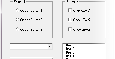
In this article, I’d like to describe how to validate empty value in controls on UserForm of Excel VBA. It’s list of controls that you can select and enter on form.
It’s assumed that OptionButtons and CheckBoxes are placed in Frame and they aren’t placed within one Frame together.

The function that validates empty value of controls on forms is called from multiple CommandButtons. Therefore, it’s reasonable to design as public function. It’s needed to add module for implementing the function. Data type of return value is Variant as following code because it returns name list of empty controls as string. It may be Boolean if you don’t have to present message box.
Option Explicit

Function CheckControls(myForm As MSForms.UserForm) As Variant
    Dim Ctrl        As MSForms.Control
    Dim CheckCnt    As Long
    Dim myCnt       As Long
    Dim CheckStr    As String
    CheckControls = False
    CheckCnt = 0
    myCnt = 0
    CheckStr = ""
    For Each Ctrl In myForm.Controls
        Select Case TypeName(Ctrl)
            Case "ComboBox"
                If Ctrl.ListIndex <> -1 Then
                    myCnt = myCnt + 1
                Else
                    CheckStr = CheckStr & Ctrl.Name & vbCrLf
                End If
            Case "Frame"
                If CheckFrame(Ctrl) Then
                    myCnt = myCnt + 1
                Else
                    CheckStr = CheckStr & Ctrl.Name & vbCrLf
                End If
            Case "ListBox"
                If Ctrl.ListIndex <> -1 Then
                    myCnt = myCnt + 1
                Else
                    CheckStr = CheckStr & Ctrl.Name & vbCrLf
                End If
            Case "TextBox"
                If Ctrl.Text <> "" Then
                    myCnt = myCnt + 1
                Else
                    CheckStr = CheckStr & Ctrl.Name & vbCrLf
                End If
            Case Else
                CheckCnt = CheckCnt - 1
        End Select
        CheckCnt = CheckCnt + 1
    Next Ctrl
    If CheckCnt = myCnt Then
        CheckControls = True
    Else
        CheckControls = CheckStr
    End If
End Function

Function CheckFrame(myFrame As MSForms.Frame) As Boolean
    Dim FrmCnt  As Long
    Dim ChkCnt  As Long
    Dim OptCnt  As Long
    Dim tmpCtrl As Control
    CheckFrame = False
    FrmCnt = 0
    ChkCnt = 0
    OptCnt = 0
    For Each tmpCtrl In myFrame.Controls
        Select Case TypeName(tmpCtrl)
            Case "CheckBox"
                If tmpCtrl.Value Then
                    ChkCnt = ChkCnt + 1
                End If
            Case "OptionButton"
                If tmpCtrl.Value Then
                    OptCnt = OptCnt + 1
                End If
        End Select
    Next tmpCtrl
    FrmCnt = FrmCnt + 1
    If FrmCnt = OptCnt Or FrmCnt <= ChkCnt Then
        CheckFrame = True
    End If
End Function
You would write the code on click event as below. You could write the procedure between "If ... Then" and "Else" statements that is activated when it has passed verification.
Option Explicit

Private Sub CommandButton1_Click()
    If TypeName(CheckControls(Me)) = "Boolean" Then

    Else
        MsgBox Prompt:=CheckControls(Me) & "Missing value above.", Title:="Empty values!"
        Exit Sub
    End If
End Sub
To tell the truth, CheckBox has interesting property. Although OptionButton tekes only TRUE or FALSE, CheckBox takes three-valued logic with NULL. It's very difficult problem for database designers because NULL brings them unexpected results in query. Three-valued logic is the greatest weakness of relational model. TripleState property, its default value is FALSE, could select whether three-valued logic would be allowed or not.
It's assumed that one or more controls are checked in Frame. If the procedure validates naked CheckBox without Frame, what happens? Whatever the value of CheckBox is, it passes verification. You shouldn't use three-valued logic to select TURE or FALSE only.
Furthermore, to allow multiple choices means that users would be allowed to not select any options more. Relation of 1:0 and 1:n are allowed, respectively. Fortunately, the situation could be avoided with careful design of choices. It's needed to be carefully treated of "Other case" that couldn't be treated as number. It's impossible to isolate and salvage data that is classified as "Others".
References:
Userform of Excel VBA as user interface
Three-valued logic (Wikipedia)
今回はフォーム上のコントロールの形式的検証のうち,未入力のコントロールをチェックするコードを紹介します.フォーム上に入力・選択可能なコントロールとしては以下が挙げられます.
オプションボタンおよびチェックボックスはフレーム内に配置してあるものとし,一つのフレーム内にオプションボタンとチェックボックスは混在していないと仮定しています.
フォーム上のコントロールの未入力のチェックは複数のコマンドボタンから共通して呼び出される機能であるため,共通化したほうがコーディングの重複をなくせます.そのため標準モジュールを追加して関数として実装することにします.下記の関数で戻り値を Variant 型にしているのは未入力のコントロール名を文字列型で受けているためです.メッセージボックスを表示する必要がなければ戻り値を Boolean 型にした方がよいでしょう.また Select case 節でコントロールの種類を群別しているため case else 節でコントロール数を減算する処理を追加していますが,If … Then … ElseIf … 節で群別すればその記述は不要になります.
Option Explicit

Function CheckControls(myForm As MSForms.UserForm) As Variant
    Dim Ctrl        As MSForms.Control
    Dim CheckCnt    As Long
    Dim myCnt       As Long
    Dim CheckStr    As String
    CheckControls = False
    CheckCnt = 0
    myCnt = 0
    CheckStr = ""
    For Each Ctrl In myForm.Controls
        Select Case TypeName(Ctrl)
            Case "ComboBox"
                If Ctrl.ListIndex <> -1 Then
                    myCnt = myCnt + 1
                Else
                    CheckStr = CheckStr & Ctrl.Name & vbCrLf
                End If
            Case "Frame"
                If CheckFrame(Ctrl) Then
                    myCnt = myCnt + 1
                Else
                    CheckStr = CheckStr & Ctrl.Name & vbCrLf
                End If
            Case "ListBox"
                If Ctrl.ListIndex <> -1 Then
                    myCnt = myCnt + 1
                Else
                    CheckStr = CheckStr & Ctrl.Name & vbCrLf
                End If
            Case "TextBox"
                If Ctrl.Text <> "" Then
                    myCnt = myCnt + 1
                Else
                    CheckStr = CheckStr & Ctrl.Name & vbCrLf
                End If
            Case Else
                CheckCnt = CheckCnt - 1
        End Select
        CheckCnt = CheckCnt + 1
    Next Ctrl
    If CheckCnt = myCnt Then
        CheckControls = True
    Else
        CheckControls = CheckStr
    End If
End Function

Function CheckFrame(myFrame As MSForms.Frame) As Boolean
    Dim FrmCnt  As Long
    Dim ChkCnt  As Long
    Dim OptCnt  As Long
    Dim tmpCtrl As Control
    CheckFrame = False
    FrmCnt = 0
    ChkCnt = 0
    OptCnt = 0
    For Each tmpCtrl In myFrame.Controls
        Select Case TypeName(tmpCtrl)
            Case "CheckBox"
                If tmpCtrl.Value Then
                    ChkCnt = ChkCnt + 1
                End If
            Case "OptionButton"
                If tmpCtrl.Value Then
                    OptCnt = OptCnt + 1
                End If
        End Select
    Next tmpCtrl
    FrmCnt = FrmCnt + 1
    If FrmCnt = OptCnt Or FrmCnt <= ChkCnt Then
        CheckFrame = True
    End If
End Function
フォーム上のコマンドボタンには下記のコードを記述します.If ... Then 節には入力値の検証に合格した際の動作を記述します.
Option Explicit

Private Sub CommandButton1_Click()
    If TypeName(CheckControls(Me)) = "Boolean" Then

    Else
        MsgBox Prompt:=CheckControls(Me) & "上記項目が未入力です", Title:="未入力エラー"
        Exit Sub
    End If
End Sub
さて,実はチェックボックスには面白い性質があります.オプションボタンでは TRUE と FALSE の 2 値しか取りませんが,チェックボックスの場合は更に NULL を加えた 3 値の真理値を取ることができます.しかしデータベース設計者にとって NULL は極めて扱いの難しい真理値であり,クエリが予想外の結果を返すことがあるためなるべく NULL を許容すべきではありません.3 値論理は関係モデルにとって急所なのです.TripleState プロパティで 3 値論理を認めるか否か変更できます.既定値は FALSE となっています.一方でオプションボタンにはそのようなプロパティは存在しません.
上記の例文ではフレーム内のチェックボックスやリストボックスの選択肢から最低でも 1 つ選択されている,という前提でチェックをかけています.では,フレーム内ではなくフォーム上にチェックボックスが存在する場合はどうでしょうか.この場合,チェックボックスの値にかかわらず検証はパスします.ですが TRUE か FALSE かを必ず選択させるために 3 値論理を導入するのは行き過ぎかと思います.
さらにチェックボックス,リストボックスいずれにも言えることですが,複数選択を許可するということは,どの選択肢も選択しないことをも許容することを意味します.つまり関係モデル上 1:n のリレーションのうち n = 0 も成り立つということです.とは言え,選択肢を注意深く設定することである程度は回避可能です.例えば年齢を 10 歳区分で区切る場合に両端の年代をどのように扱うかや,年収を 100 万円単位で区切る場合に最小群と最大群をどう設定するかなどです.数値で扱えない選択項目の場合,「その他」をどこまで許容するか,慎重に設計しなければなりません.一旦「その他」に放り込まれたデータを後から切り分けて取り出すことは不可能です.必要な項目を網羅した上でこれ以上はどう考えても不要である場合にのみ「その他」とする,つまり漏れがないように選択肢を設定すべきです.
参照:
インターフェースとしてのEXCEL VBAによるユーザーフォーム
Three-valued logic (Wikipedia)


")
")
!2!}")

 = S_0(t)^{\exp(R-R_0)}")
 = A \cap \neg B")